Section 1 – Research Questions

Question 1: Can we predict the global score of the student using their Quantitative Reasoning and Critical Reading?

Question 2: Can we predict the global score of the student using their Quantitative Reasoning and Critical Reading with School Nature as dummy variable?

Section 2 – Dataset

• Representativeness: The representativeness of the sample is determined by the randomness of the sample and its ability to represent the whole population
• Statistics of variable of interest: The dataset is analysed and some variables of interest for the understanding of the Research Questions are selected.

The summary statistics of the variables of interest are shown below:

Summary Statistics:

> var_of_interest <- c('gender','revenue','school_nat','cr_pro','qr_pro','g_sc')
> summary(s_perform[var_of_interest])
    gender            revenue           school_nat            cr_pro          qr_pro            g_sc      
    Length:12406       Length:12406       Length:12406       Min.   :  1.0   Min.   :  1.00   Min.   : 37.0  
    Class :character   Class :character   Class :character   1st Qu.: 42.0   1st Qu.: 65.00   1st Qu.:147.0  
    Mode  :character   Mode  :character   Mode  :character   Median : 67.0   Median : 85.00   Median :163.0  
                                                            Mean   : 62.2   Mean   : 77.42   Mean   :162.7  
                                                            3rd Qu.: 86.0   3rd Qu.: 96.00   3rd Qu.:179.0  
                                                            Max.   :100.0   Max.   :100.00   Max.   :247.0  
                        

• Visualization of the Variables: To further understand the data of the variables of interest, we do some visualizations to understand the distribution of the data.

Output:

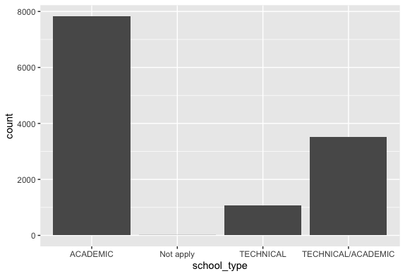
school_type analysis

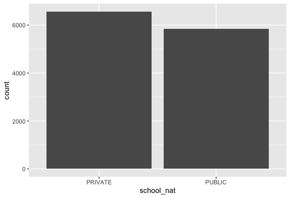
School Nature analysis

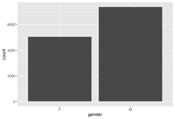
Gender wise analysis

Revenue wise analysis

>

Observations:

• School type analysis: It shows an outlier ‘Not apply’ which is in very few number only 5 records, so we can ignore those outliers.
• School Nature analysis: It shows the classification of 12,411 records based on the school they attended before engineering. It can be observed there is only a slight difference between the public and private institutes.
• Gender wise analysis: It shows the classification of male and female pursuing engineering. It can be observed Females are considerably less compared to male.

• Assessing Normality: The normality of variables like ENG_S11, ENG_PRO, CR_S11, CR_PRO are determined as it is necessary for further analysis of the dataset and building a model.
  • For g_sc:

    Inspection:

    Descriptive Inspection:

    > pastecs::stat.desc(s_perform$g_sc, basic=F)
        median         mean      SE.mean CI.mean.0.95          var      std.dev     coef.var 
    163.0000000  162.7153797    0.2074881    0.4067090  534.0948009   23.1104911    0.1420302 
    > g_scskew<-semTools::skew(s_perform$g_sc)
    > g_sckurt<-semTools::kurtosis(s_perform$g_sc)
    > g_scskew[1]/g_scskew[2]
    skew (g1) 
    -4.322486 
    > g_sckurt[1]/g_sckurt[2]
    Excess Kur (g2) 
        -1.715517 
    > g_sc<- abs(scale(s_perform$g_sc))
    > FSA::perc(as.numeric(g_sc), 1.96, "gt")
    [1] 4.05449
    > FSA::perc(as.numeric(g_sc), 3.29, "gt")
    [1] 0.1531517
                                                

    Output: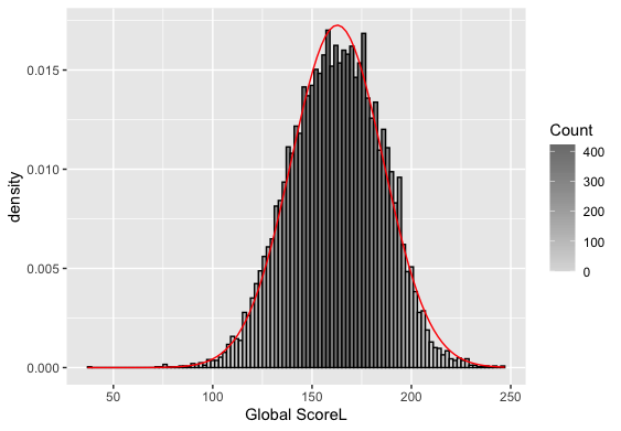

    Result:

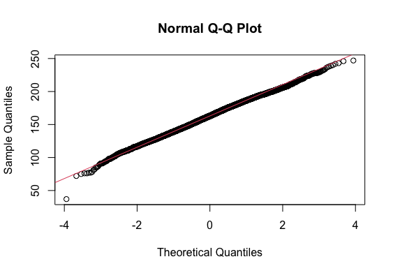
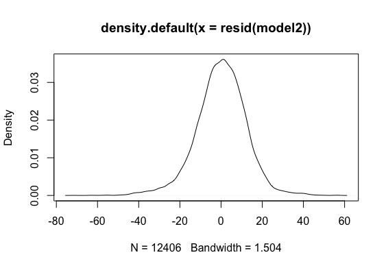
    • From the density curve and the q-q plot we can assume through visual inspection that the vairable maybe normal. But cannot confirm it because of the slight skew caused by outliers so we do descrpitive analysis to make sure that the outliers are within the expected limit.
    • From the above summary statistics we can observe that skew is -4.3, which is (>2) and not acceptable, so we look further into it by finding out the outliers that are contributing the skew.
    • Since our dataset has more than 80 records, we use +/- 3.29 as our measure. In that case we have 0.15% of values fall outside +/- 3.29. Therefore, it is okay to treat this as Normal.

  Reporting Normality for g_sc:

  g_sc was assessed for normality. Visual inspection of the histogram and QQ-Plot identified some issues with skewness and kurtosis. The standardised score for kurtosis (-1.72) can be considered acceptable using the criteria proposed by West, Finch and Curran (1996), but the standardised score for skewness (-4.32) was outside the acceptable range. However 100% of standardised scores for g_sc fall within the bounds of +/- 3.29, using the guidance of Field, Miles and Field (2013) the data can be considered to approximate a normal distribution.

• Missing Values:
  Descriptive Inspection:

  > na_count
  cod_s11 gender edu_father edu_mother occ_father occ_mother stratum sisben people_house ...10 internet tv
  1       0      0          0          0          0          0       0      0            0   100        0  0
  computer washing_mch mic_oven car dvd fresh phone mobile revenue job school_name school_nat school_type
  1        0           0        0   0   0     0     0      0       0   0           0          0           0
  mat_s11 cr_s11 cc_s11 bio_s11 eng_s11 cod_spro university academic_program qr_pro cr_pro cc_pro eng_pro
  1       0      0      0       0       0        0          0                0      0      0      0       0
  wc_pro fep_pro g_sc percentile X2nd_decile quartile sel sel_ihe
  1      0       0    0          0           0        0   0       0
  
  s_perform <- filter(s_perform, s_perform$school_type !='Not apply')
  s_perform
                                      

  Result:

  • From the output above, we can conclude that the dataset doesn’t have any significant missing values except for one column “…10” which doesn’t have any significant meaning. So we ignore that as we are not interested in that column for our analysis.
  • The outlier records with 'not apply' are removed here to avoid their influence on the model

Section 3 - Results

Section 3.1 - Statistical evidence

• Checking for correlation between predictors and dependent variable.

            The predictors are chosen with the help of a correlation test, this is done to identify some kind of relationship between the predictor and the dependent variable. If there exists a moderate/high correlation then we can assume that variable to be a predictor.

• Correlation between global score and Quantitative reasoning

  Null Hypothesis: The population correlation coefficient between g_sc and qr_pro is equal to a hypothesized value (=0 indicating no linear correlation)
  Alternate Hypothesis: The population correlation coefficient between g_sc and qr_pro is not equal (or less than, or greater than) the hypothesized value(indicating linear correlation)

   

  Descriptive Inspection:

      > stats::cor.test(s_perform$g_sc, s_perform$qr_pro, method='pearson')
  
      Pearson's product-moment correlation
  
  data:  s_perform$g_sc and s_perform$qr_pro
  t = 109.1, df = 12404, p-value < 2.2e-16
  alternative hypothesis: true correlation is not equal to 0
  95 percent confidence interval:
      0.6906862 0.7086488
  sample estimates:
          cor 
  0.6997781 
                                      

  Output: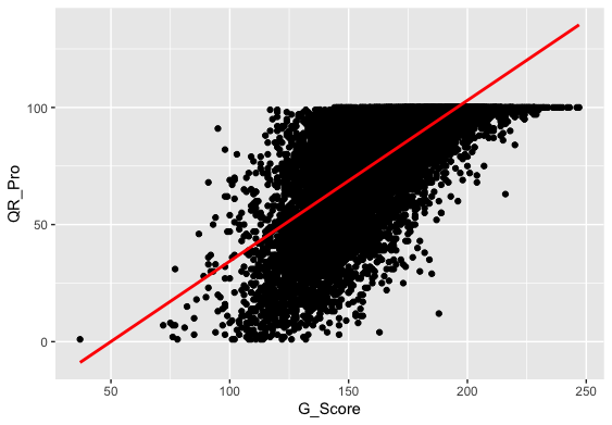

  Result:

  We can observe from the graph that there is a moderate positive linear correlation, which implies we have satisfied our assumptions for pearson test they are:

  • Correlation requires that both variables be quantitative.
  • Correlation describes linear relationships.

  
  From Pearson correlation,we get a correlation of 0.70, which means the effect size is medium(Acc. to cohen's effect size heuristic).
  Assuming our alpha level = 0.05, our p-value(0.001) < 0.05 => The correlation is statistically significant.
  And so we have evidence to reject null hypothesis in favour of the alternate which is there is a relationship between g_sc and qr_pro. So, we can use qr_pro as one of the predictors

  Report for Correlation between global score and Quantitative reasoning:

  The relationship between g_sc(global score achieved by students) and qr_pro(Quantitative reasoning achieved in University) was investigated using a Pearson correlation. A positive correlation was found(r=0.70,n=12404,p< 0.001).

• Correlation between global score and Critical Reading:

  Null Hypothesis: The population correlation coefficient between g_sc and cr_pro is equal to a hypothesized value (=0 indicating no linear correlation)
  Alternate Hypothesis: The population correlation coefficient between g_sc and cr_pro is not equal (or less than, or greater than) the hypothesized value(indicating linear correlation)

  Descriptive Inspection:

      > stats::cor.test(s_perform$g_sc, s_perform$cr_pro, method='pearson')
  
      Pearson's product-moment correlation
  
  data:  s_perform$g_sc and s_perform$cr_pro
  t = 141.79, df = 12404, p-value < 2.2e-16
  alternative hypothesis: true correlation is not equal to 0
  95 percent confidence interval:
      0.7796011 0.7930323
  sample estimates:
          cor 
  0.7864097 
                                      

  Output: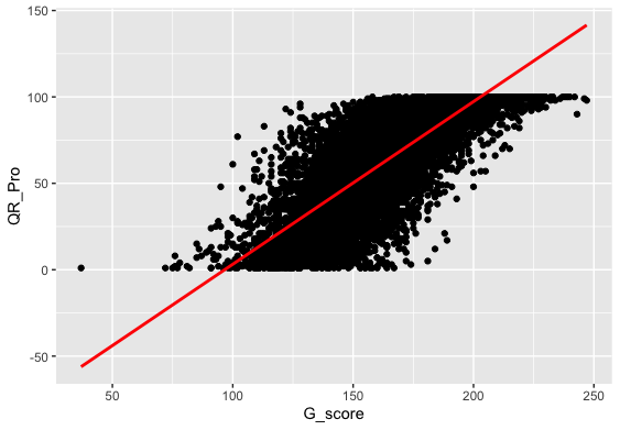

  Result:

  We can observe from the graph that there is a high positive linear correlation, which implies we have satisfied our assumptions for pearson test they are:

  • Correlation requires that both variables be quantitative.
  • Correlation describes linear relationships.

  
  From Pearson correlation,we get a correlation of 0.79, which means the effect size is large(Acc. to cohen's effect size heuristic).
  Assuming our alpha level = 0.05, our p-value(0.001) < 0.05 => The correlation is statistically significant.
  And so we have evidence to reject null hypothesis in favour of the alternate which is there is a relationship between g_sc and cr_pro. So, we can use cr_pro as one of the predictors

  Report for Correlation between global score and Critical Reading:

  The relationship between g_sc(global score achieved by students) and cr_pro(Critical Reading achieved in University) was investigated using a Pearson correlation. A strong positive correlation was found(r=0.79,n=12404,p< 0.001).

• T-test for differential variable.

               The t test tells you how significant the differences between groups are; In other words it lets you know if those differences (measured in means) could have happened by chance.

  Hypothesis (Two-tailed):

  Null Hypothesis H0: There is no difference in mean g_sc score between those who went to a private and public school.

  Alternate Hypothesis HA: There is a difference in mean g_sc score between those who went to a private and public school.

  Output:

      > psych::describeBy(s_perform$g_sc, s_perform$school_nat, mat=TRUE)
      item  group1 vars    n     mean       sd median  trimmed     mad min max range        skew    kurtosis
  X11    1 PRIVATE    1 6560 168.2293 22.81689    170 168.7494 23.7216  37 247   210 -0.20320838  0.02354186
  X12    2  PUBLIC    1 5846 156.5281 21.83817    157 156.5667 22.2390  72 228   156 -0.05215938 -0.01912125
              se
  X11 0.2817115
  X12 0.2856189
  > car::leveneTest(g_sc ~ school_nat, data=s_perform)
  Levene's Test for Homogeneity of Variance (center = median)
              Df F value    Pr(>F)    
  group     1  12.514 0.0004054 ***
          12404                      
  ---
  Signif. codes:  0 ‘***’ 0.001 ‘**’ 0.01 ‘*’ 0.05 ‘.’ 0.1 ‘ ’ 1
  > stats::t.test(g_sc ~ school_nat,var.equal=FALSE,data=s_perform)
  
      Welch Two Sample t-test
  
  data:  g_sc by school_nat
  t = 29.168, df = 12341, p-value < 2.2e-16
  alternative hypothesis: true difference in means is not equal to 0
  95 percent confidence interval:
      10.91485 12.48758
  sample estimates:
  mean in group PRIVATE  mean in group PUBLIC 
                  168.2293              156.5281 
  
  Since homogeneity failed we are setting var.equal to FALSE as there is no equal means
  
  > res <- stats::t.test(g_sc ~ school_nat,var.equal=FALSE,data=s_perform)
  > effcd=round((2*res$statistic)/sqrt(res$parameter),2)
  > effectsize::t_to_d(t = res$statistic, res$parameter)
      d |       95% CI
  -------------------
  0.53 | [0.49, 0.56]
  > effes=round((res$statistic*res$statistic)/((res$statistic*res$statistic)+(res$parameter)),3)
  > effes
      t 
  0.064 
                                  

  Result:

  • Levene's Test: For homogeneity of variance Null Hypothesis: All variances are equal. Alternate Hypothesis: All variances are not equal. From the test, we can see Pr(>F) is 0.01,which is less than 0.05, so it is statistically significant, thus rejecting null hypothesis(Homogeneity).
  • Cohens-d value = 0.53, which implies a medium effect size.
  • eta value = 0.064, which implies a medium effect size.
  • Since the test was statistically significant it implies that the variable school_nat could act as a predictor for g_sc.

  Report for T-test of school_nat variable:

  "An independent-samples t-test was conducted to compare the mean scores of g_sc for students who studied in Public and Private schools. A significant difference in the scores for g_sc was found ( M=168.23, SD= 22.8 for students studied in Private schools, M= 156.53,SD= 21.83 for students who studied in Public Schools),(t(12404)= 29.17, p = 0.01). A medium effect size was also indicated by Cohen's d value (0.53)."

Section 3.2 – Model 1

Research Question : Can we predict the global score of the student using their Quantitative Reasoning and Critical Reading?

Null Hypothesis: The values of g_sc cannot be predicted with the predictor variables(cr_pro, qr_pro) using Multiple linear Regression.

Alternate Hypothesis: : The values of g_sc can be predicted with the predictor variables(cr_pro, qr_pro) using Multiple linear Regression.

Descriptive Inspection:

> model1<-lm(s_perform$g_sc~s_perform$qr_pro+s_perform$cr_pro)

> stargazer(model1, type="text") 

=================================================
                            Dependent variable:     
                    -----------------------------
                                g_sc             
-------------------------------------------------
qr_pro                        0.380***           
                                (0.006)           
                                                    
cr_pro                        0.480***           
                                (0.005)           
                                                    
Constant                     103.484***          
                                (0.398)           
                                                    
-------------------------------------------------
Observations                   12,406            
R2                              0.712            
Adjusted R2                     0.712            
Residual Std. Error      12.401 (df = 12403)     
F Statistic         15,341.490*** (df = 2; 12403)
=================================================

> lm.beta(model1)

Call:
lm(formula = s_perform$g_sc ~ s_perform$qr_pro + s_perform$cr_pro)

Standardized Coefficients::
        (Intercept) s_perform$qr_pro s_perform$cr_pro 
        0.0000000        0.3725515        0.5740398

> vifmodel
s_perform$qr_pro s_perform$cr_pro 
        1.481366         1.481366 
> #Tolerance
> 1/vifmodel
s_perform$qr_pro s_perform$cr_pro 
        0.6750525        0.6750525
                                
                            

Result:

• The p-value indicates our model is significant, so we can reject the null hypothesis and accept the alternate hypothesis that the values of g_sc can be predicted with the predictor variables(cr_pro, qr_pro) using Multiple linear Regression.
• Increase marks in qr_pro and cr_pro appears to be associated with increase marks in g_sc.
• The F statistic looks at whether the model as whole is statistically significant.
• In our case adjusted r 2 value 0.712, which means around 71.2% of the variance g_sc can be explained by cr_pro and qr_pro.
• Our linear regression model is Predicted g_sc = 103 + 0.38*qr_pro + 0.48*cr_pro
• In our case using the standardised coefficents our model equation becomes: Predicted g_sc = 0 + 0.373*qr_pro + 0.574*cr_pro

---

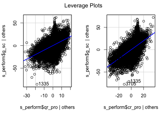
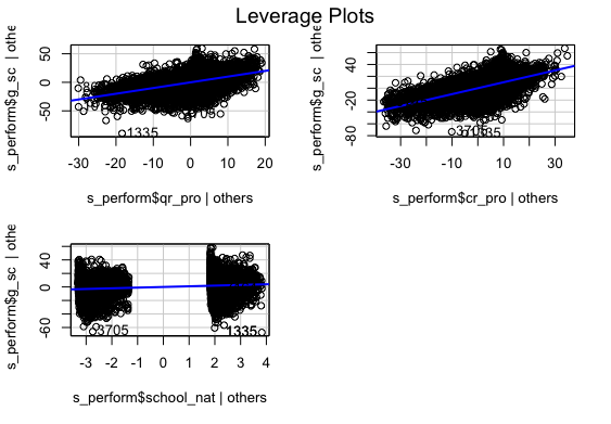
Assumptions:

Output:

Cooks plot

Leverage

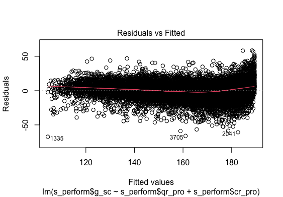
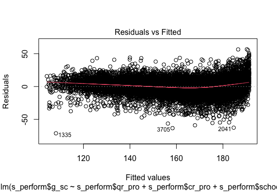
Ressidual Fit

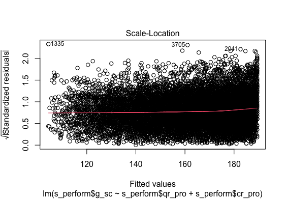
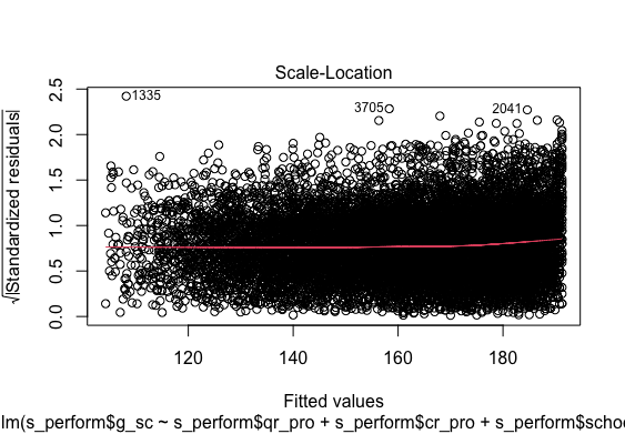
Standard Residual Fit

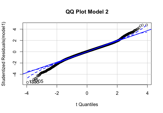
QQ Error distribution

Histogram error distribution

Result:

• It can be observed that all the points are less than 1, So we don't have to worry about the outliers
• We can see that there is no pattern and points are equally distributed, therefore homoscedasticity is not an concern
• Minimum and Maximum value is within the acceptable range(-3.29,+3.29) hence we do not have outliers. Though the red lines are slightly distorted but this is not a huge problem
• We can see that the errors are normally distributed
• Both collinearity and tolerance were with the acceptable limits (VIF < 2.5 and tolerance > 0.4). So, we have no issues with Multi collinearity.

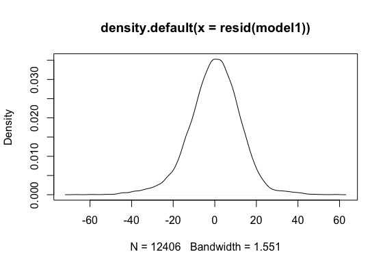
Reporting Multiple linear Regression(Model 1):

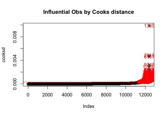
Multiple regression analysis was conducted to determine the global scores(g_sc). Scores of Quantitative Reasoning and Critical Reading were used as predictor variables. Examination of the histogram, normal P-P plot of standardised residuals and the scatterplot of the dependent variable, and standardised residuals showed that some outliers existed. However, examination of the standardised residuals showed that some could be considered to have undue influence (95% within limits of -1.96 to plus 1.96 and none with Cook’s distance >1 as outlined in Field (2013). Examination for multicollinearity showed that the tolerance and variance influence factor measures were within acceptable levels (tolerance >0.4, VIF < 2.5 ) as outlined in Tarling (2008). The scatterplot of standardised residuals showed that the data met the assumptions of homogeneity of variance and linearity. The data also meets the assumption of non-zero variances of the predictors.

Section 3.3 – Model 2

Research Question : Can we predict the global score of the student using their Quantitative Reasoning and Critical Reading with School Nature as dummy variable?

 

Differential effect

• We use the variable school_nat as a predictor, since it is a categorical type we use it as a dummy variable to understand the differential effect of the global_scores of students studied in Private and Public schools.
• Here, 0 (reference category, Private) and 1 (category of interest, Public)

Null Hypothesis The values of g_sc cannot be predicted with the predictor variables(cr_pro, qr_pro, school_nat) using Multiple linear Regression.

Alternate Hypothesis: : The values of g_sc can be predicted with the predictor variables(cr_pro, qr_pro, school_nat) using Multiple linear Regression.

Descriptive Inspection:

> model2<-lm(s_perform$g_sc~s_perform$qr_pro+s_perform$cr_pro+s_perform$school_nat)

> stargazer(model2, type="text") #Tidy output of all the required stats

=================================================
                            Dependent variable:     
                    -----------------------------
                                g_sc             
-------------------------------------------------
qr_pro                        0.368***           
                                (0.006)           
                                                    
cr_pro                        0.471***           
                                (0.005)           
                                                    
school_natPUBLIC              -5.134***          
                                (0.222)           
                                                    
Constant                     107.329***          
                                (0.424)           
                                                    
-------------------------------------------------
Observations                   12,406            
R2                              0.724            
Adjusted R2                     0.724            
Residual Std. Error      12.141 (df = 12402)     
F Statistic         10,847.740*** (df = 3; 12402)
=================================================
Note:                 *p< 0.1; **p< 0.05; ***p< 0.01

> lm.beta(model2)

Call:
lm(formula = s_perform$g_sc ~ s_perform$qr_pro + s_perform$cr_pro + 
    s_perform$school_nat)

Standardized Coefficients::
                (Intercept)           s_perform$qr_pro           s_perform$cr_pro s_perform$school_natPUBLIC 
                    0.0000000                  0.3614803                  0.5634178                 -0.1109039

            

Result:

• The p-value indicates our model is significant, so we can reject the null hypothesis and accept the alternate hypothesis that the values of g_sc can be predicted with the predictor variables(cr_pro, qr_pro,school_nat) using Multiple linear Regression.
• Increased marks in qr_pro and cr_pro appears to be associated with increase marks in g_sc.
• The F statistic looks at whether the model as whole is statistically significant.
• Our linear regression model is Predicted g_sc = 103 + 0.368*qr_pro + 0.471*cr_pro – 5.134*school_natPUBLIC
• In our case using the standardised coefficients our model equation becomes: Predicted g_sc = 0 + 0.361*qr_pro + 0.563*cr_pro - 0.11* school_natPUBLIC
• When we calculate the equation for Public and Private schools:
  Public = 0+0.361+0.563-0.11=0.814
  Private=0+0.361+0.563 =0.924
• We can see a small difference between the group yes and no.
• We can see a slight change in the coefficent compared to model 1.
• In our case adjusted r 2 value 0.724, which means around 72.4% of the variance g_sc can be explained by cr_pro and qr_pro when a dummy variable school_nat is added. An increase compared to model 1.

---

Assumptions:

Output:

Cooks plot

Leverage

Ressidual Fit

Standard Residual Fit

QQ Error distribution

Histogram error distribution

Result:

• It can be observed that all the points are less than 1, So we don't have to worry about the outliers
• We can see that there is no pattern and points are equally distributed, therefore homoscedasticity is not an concern
• Minimum and Maximum value is within the acceptable range(-3.29,+3.29) hence we do not have outliers. Though the red lines are slightly distorted but this is not a huge problem
• We can see that the errors are normally distributed
• Both collinearity and tolerance were with the acceptable limits (VIF < 2.5 and tolerance > 0.4). So, we have no issues with Multi collinearity.
• The differential effect in the global scores can be see between the students who studied in Public and Private.

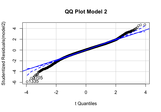
Reporting Multiple linear Regression(Model 2):

Multiple regression analysis was conducted to determine the global scores(g_sc). Scores of Quantitative Reasoning and Critical Reading were used as predictor variables. In order to include the School Nature in the regression model it was recorded dummy variable school_nat (0 for Private, 1 for Public).Examination of the histogram, normal P-P plot of standardised . Examination of the histogram, normal P-P plot of standardised residuals and the scatterplot of the dependent variable, and standardised residuals showed that some outliers existed. However, examination of the standardised residuals showed that some could be considered to have undue influence (95% within limits of -1.96 to plus 1.96 and none with Cook’s distance >1 as outlined in Field (2013). Examination for multicollinearity showed that the tolerance and variance influence factor measures were within acceptable levels (tolerance >0.4, VIF < 2.5 ) as outlined in Tarling (2008). The scatterplot of standardised residuals showed that the data met the assumptions of homogeneity of variance and linearity. The data also meets the assumption of non-zero variances of the predictors.

Section 3.3 – Model comparison

> stargazer(model1, model2, type="text") 

===============================================================================
                                        Dependent variable:                    
                    -----------------------------------------------------------
                                                g_sc                            
                                    (1)                           (2)             
-------------------------------------------------------------------------------
qr_pro                        0.380***                      0.368***           
                                (0.006)                       (0.006)           
                                                                                
cr_pro                        0.480***                      0.471***           
                                (0.005)                       (0.005)           
                                                                                
school_natPUBLIC                                            -5.134***          
                                                                (0.222)           
                                                                                
Constant                     103.484***                    107.329***          
                                (0.398)                       (0.424)           
                                                                                
-------------------------------------------------------------------------------
Observations                   12,406                        12,406            
R2                              0.712                         0.724            
Adjusted R2                     0.712                         0.724            
Residual Std. Error      12.401 (df = 12403)           12.141 (df = 12402)     
F Statistic         15,341.490*** (df = 2; 12403) 10,847.740*** (df = 3; 12402)
===============================================================================
Note:                                               *p< 0.1; **p < 0.05; ***p < 0.01
                                
                            

Section 4 – Discussion/Conclusion

• Research question 1, was successfully answered by creating a model to predict the global scores and the necessary steps required to build said model are followed and the model is tested.
• Research question 2, was successfully answered by creating a model to predict the global scores and the differential effect of school_nat has been analysed and added to the model and the model is tested.
• New research questions can be developed using other variables in the dataset like the eng_s11, qr_s11, mat_s11 can be used to predict the eng_pro, qr_pro.