Explore

Descriptive Statistics

Summary Statistics

Measures of Central Tendency:
- Descriptive Statistics for numerical data
- A single number which can represent the whole data and around which the other data tend to cluster
- Measured using 3 methods: Mean,Median,Mode
- Mean: It is the arithmetic average of the values in a feature in sample.
- Median: It is the middle value from all the values in a feature in the sample given that the value of the feature are arranged in some kind of order (ascending/descending). If the number of values are even, the median is the average of the middle two values.
  - Not affected by the outliers in the data set. An outlier is a data point that is radically “distant” or “away” from common trends of values in a given set. It does not represent a typical number in the set.
  - The concept of the median is intuitive thus can easily be explained as the center value.
  - Each set has a unique median value.
  - Its value is perceived as it is. It cannot be utilized for further algebraic treatment.
  It is more susceptible to outliers than mean of measuring central tendancy.
- Mode: It is the most frequently occured measure from the feature in the sample.
  It is more insensitive to large changes to the sample Note: If a distribution has two modes then it is known as bimodal.
  - Just like the median, the mode is not affected by outliers.
  - Useful to find the most “popular” or common item. This includes data sets that do not involve numbers.
  - If the feature contains no repeating values or more repeating value ,this is meaningless
  It is more used in case of Qualitative numerical values like nominal/Ordinal.
Measures of Dispersion:

Dispersion/Vairability

Reported with the measurement of central tendancy

Variability measures the amount of scatter in the dataset

Gives more insight on the outliers.
- Range: The difference between the largest and smallest values in the feature.
- Variance:This method uses the deviation of the values from the mean of the feature.
  Since the difference between mean and the value may give negative values, summing it can cancel it, so we square it and then add. And then find the average.
  For the average, we divide the sum with the degrees of Freedom. Note: For sample, through experiments it is found that the degree of freedom is N-1
  For population, we divide the sum with the total number of values in the set(N).
- Standard deviation: It is the square-root of the variance.This is the more common measure since it makes it will be in the units of measurement rather than squared units of measurement – so is more intuitive.
  The larger the value the more spread out around the mean the data is, smaller means less spread. The Empirical Rule:The 68-95-99.7 Rule
  - 68% of the observations fall within σ of the mean µ.
  - 95% of the observations fall within 2σ of the mean µ.
  - 99.7% of the observations fall within 3σ of the mean µ.
- IQR: Interquartile range (IQR) is the range of the middle half of the data.
Degrees of Freedom: Degrees of freedom of an estimate is the number of independent pieces of information that went into calculating the estimate.

Measures of shape:

The shape of a distribution is measured using its skewness.

Skewed: When the data points cluster more toward one side of the scale than the other, creating a curve that is not symmetrical. It could be both positively skewed or negatively skewed.
- Positively skewed:When the data points cluster towards the left leading a tail on the right.It means that the outliers are to the right (long tail to the right).
- Negatively skewed:When the data points cluster towards the right leading a tail on the left. It means that the outliers are to the left.
- Kurtosis:It shows the heaviness of the tail,which can be divided as Leptokurtic = heavy tails (more scores in the tails), Platykurtic = light tails (more scores in the middle).

The dependance between two variables are measured using correlation.

Exploring & Analysing the dataset

Basic summary of Variables of Interest:

Code:


                                
                                    >var_of_interest <- c('Pstatus','schoolsup.m','internet','higher.m','age','mG1','mG2','mG3','sex')
                                    >summary(s_perform[var_of_interest])

Result:


                                Pstatus          schoolsup.m          internet           higher.m              age             mG1       
Length:382         Length:382         Length:382         Length:382         Min.   :15.00   Min.   : 3.00  
Class :character   Class :character   Class :character   Class :character   1st Qu.:16.00   1st Qu.: 8.00  
Mode  :character   Mode  :character   Mode  :character   Mode  :character   Median :17.00   Median :10.50  
                                                                            Mean   :16.59   Mean   :10.86  
                                                                            3rd Qu.:17.00   3rd Qu.:13.00  
                                                                            Max.   :22.00   Max.   :19.00  
        mG2             mG3       
Min.   : 0.00   Min.   : 0.00  
1st Qu.: 8.25   1st Qu.: 8.00  
Median :11.00   Median :11.00  
Mean   :10.71   Mean   :10.39  
3rd Qu.:13.00   3rd Qu.:14.00  
Max.   :19.00   Max.   :20.00

Assesing Normality:

Generating Plots:
- A visual inspection based on the histogram and normal distribution curve
- Q-Q plot:A scatterplot created by plotting two sets of quantiles against one another. If both sets of quantiles came from the same distribution, we should see the points forming a line that’s roughly straight.
Generating Summary Statistics:
- A numerical inspection with the measures of skewness and kurtosis with standardised score.
Conducting Tests for Normality:
- Shapiro-Wilks (sample size 50 up to 2000)
- Kolmogrov-Smirnoff (larger samples >50)

Different tests for different categories:

Comparing	Dependent Variable	Independent Variable	Parametric Tests	Non-Parametric Tests
The means of two INDEPENDENT groups	Continuous/ scale	Categorical/ nominal	Independent t-test	Mann-Whitney test
The means of 2 paired (matched) samples e.g. weight before and after a diet for one group of subjects	Continuous/ scale	Time variable (time 1 = before, time 2 = after)	Paired t-test	Wilcoxon signed rank test
The means of two INDEPENDENT groups	Continuous/ scale	Categorical/ nominal	Independent t-test	Mann-Whitney test
The means of 3+ independent groups	Continuous/ scale	Categorical/ nominal	Independent t-test	Mann-Whitney test
The means of two INDEPENDENT groups	Continuous/ scale	Categorical/ nominal	One-way ANOVA	Kruskal-Wallis test
The 3+ measurements on the same subject	Continuous/ scale	Time variable	Repeated measures ANOVA	Friedman test
Relationship between 2 continuous variables	Continuous/ scale	Continuous/ scale	Pearson’s Correlation Coefficient	Spearman’s Correlation Coefficient (also use for ordinal data)
Predicting the value of one variable from the value of a predictor variable	Continuous/ scale	Any	Simple Linear Regression
Assessing the relationship between two categorical variables	Categorical/ nominal	Categorical/ nominal		Chi-squared test

Assesing Normality for the continous variables mG2,mG3:

Visual inspection:

Code:


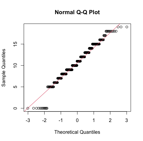
                                            #Histogram of mG2
gg <- ggplot(s_perform, aes(x=s_perform$mG2))

#Change the label of the x axis
gg <- gg + labs(x="maths grade 2")

#manage binwidth and colours
gg <- gg + geom_histogram(binwidth=2, colour="black", aes(y=..density..,
        fill=..count..))
gg <- gg + scale_fill_gradient("Count", low="#DCDCDC", high="#7C7C7C")

#adding a normal curve
#use stat_function to compute a normalised score for each value of mG2
#pass the mean and standard deviation
#use the na.rm parameter to say how missing values are handled
gg <- gg + stat_function(fun=dnorm, color="red",args=list(mean=mean(
        s_perform$mG2, na.rm=TRUE), sd=sd(s_perform$mG2, na.rm=TRUE)))

#to display the graph request the contents of the variable be shown
gg


qqnorm(s_perform$mG2)
qqline(s_perform$mG2, col=2)

Output: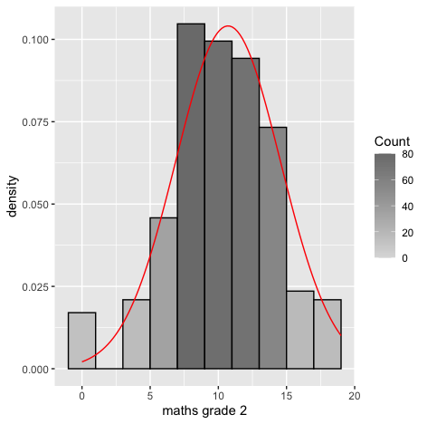

Result:

From the density curve and the q-q plot we can assume through visual inspection that the vairable maybe normal. But cannot confirm it because of the slight skew caused by outliers so we do descrpitive analysis to make sure that the outliers are within the expected limit.

For mg3

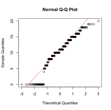
Code:


                                            #mG3

gg <- ggplot(s_perform, aes(x=s_perform$mG3))
gg <- gg + labs(x="maths grade 3")
gg <- gg + geom_histogram(binwidth=2, colour="black", aes(y=..density..,
        fill=..count..))
gg <- gg + scale_fill_gradient("Count", low="#DCDCDC", high="#7C7C7C")
gg <- gg + stat_function(fun=dnorm, color="red",args=list(mean=mean(
        s_perform$mG3, na.rm=TRUE), sd=sd(s_perform$mG3, na.rm=TRUE)))
gg

#qq plot
qqnorm(s_perform$mG3)
qqline(s_perform$mG3, col=2)

Output: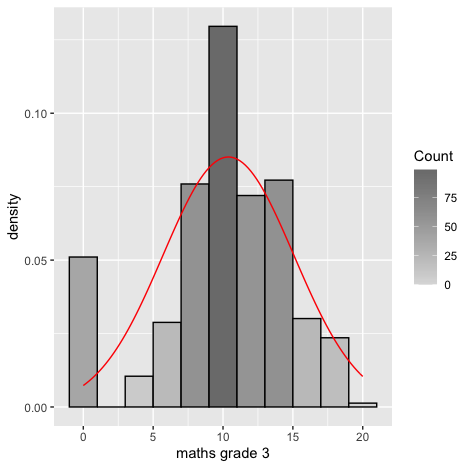

Result:

Descriptive inspection:

Code:


                                            pastecs::stat.desc(s_perform$mG2, basic=F)

#We can make our decision based on the value of the standardised score for skew and kurtosis
#We divide the skew statistic by the standard error to get the standardised score
#This will indicate if we have a problem
mG2skew<-semTools::skew(s_perform$mG2)
mG2kurt<-semTools::kurtosis(s_perform$mG2)
mG2skew[1]/mG2skew[2]

mG2kurt[1]/mG2kurt[2]

#and by calculating the percentage of standardised scores for the variable itself that are outside our acceptable range
#This will tell us how big a problem we have
# Calculate the percentage of standardised scores that are greated than 1.96
# the perc function which is part of the FSA package which calculate the percentage that are within a range - you can look for greater than "gt", greater than or equal "geq", "gt", less than or equal "leq",  or less than "lt"),
# scale is a function that creates z scores, abs gets absolute value

zmG2<- abs(scale(s_perform$mG2))

FSA::perc(as.numeric(zmG2), 1.96, "gt")
FSA::perc(as.numeric(zmG2), 3.29, "gt")

Output:


                                        median         mean      SE.mean CI.mean.0.95          var      std.dev     coef.var 
11.0000000   10.7120419    0.1960908    0.3855557   14.6885160    3.8325600    0.3577805 
                                        
                                        > mG2skew[1]/mG2skew[2]
skew (g1) 
-3.193143 
                                        
                                        >mG2kurt[1]/mG2kurt[2]
Excess Kur (g2) 
2.023209 
                                        
                                        > FSA::perc(as.numeric(zmG2), 1.96, "gt")
[1] 4.188482
                                        
                                        > FSA::perc(as.numeric(zmG2), 3.29, "gt")
[1] 0

Result:


                                                    
                                                From the above summary statistics we can observe that skew is 
                                                -3.2, which is (>2) and not acceptable, so we look further
                                                into it by finding out the outliers that are contributing
                                                the skew.
                                                    
                                                    
                                                Since our dataset has more than 80 records, we use +/- 3.29 as our measure.
                                                In that case we have 0% of values fall outside +/- 3.29. Therefore, it is 
                                                okay to treat this as Normal.

Reporting Normality for mG2:

mG2 was assessed for normality. Visual inspection of the histogram and QQ-Plot identified some issues with skewness and kurtosis. The standardised score for kurtosis (2.02) can be considered acceptable using the criteria proposed by West, Finch and Curran (1996), but the standardised score for skewness (-3.19) was outside the acceptable range. However 100% of standardised scores for mG2 fall within the bounds of +/- 3.29, using the guidance of Field, Miles and Field (2013) the data can be considered to approximate a normal distribution.

For mg3

Code:


                                            #mG3

pastecs::stat.desc(s_perform$mG3, basic=F)

mG3skew<-semTools::skew(s_perform$mG3)
mG3kurt<-semTools::kurtosis(s_perform$mG3)
mG3skew[1]/mG3skew[2]

mG3kurt[1]/mG3kurt[2]

zmG3<- abs(scale(s_perform$mG3))

FSA::perc(as.numeric(zmG3), 1.96, "gt")
FSA::perc(as.numeric(zmG3), 3.29, "gt")

Output:


                                            > pastecs::stat.desc(s_perform$mG3, basic=F)
median         mean      SE.mean CI.mean.0.95          var      std.dev     coef.var 
11.0000000   10.3874346    0.2398202    0.4715368   21.9702354    4.6872418    0.4512415 
                                            
                                            >mG3skew[1]/mG3skew[2]
skew (g1) 
-5.63212 
                                            
                                            > mG3kurt[1]/mG3kurt[2]
Excess Kur (g2) 
1.108522 
                                            
                                            >FSA::perc(as.numeric(zmG3), 1.96, "gt")
[1] 10.4712
                                            
                                            > FSA::perc(as.numeric(zmG3), 3.29, "gt")
[1] 0

Result:


                                                    
                                                From the above summary statistics we can observe that skew is 
                                                -5.63, which is (>2) and not acceptable, so we look further
                                                into it by finding out the outliers that are contributing
                                                the skew.
                                                    
                                                    
                                                Since our dataset has more than 80 records, we use +/- 3.29 as our measure.
                                                In that case we have 0% of values fall outside +/- 3.29. Therefore, it is 
                                                okay to treat this as Normal.

Reporting Normality for mG3:

mG3 was assessed for normality. Visual inspection of the histogram and QQ-Plot identified some issues with skewness and kurtosis. The standardised score for kurtosis (1.11) can be considered acceptable using the criteria proposed by West, Finch and Curran (1996), but the standardised score for skewness (-5.63) was outside the acceptable range. However 100% of standardised scores for mG3 fall within the bounds of +/- 3.29, using the guidance of Field, Miles and Field (2013) the data can be considered to approximate a normal distribution.

From the above analysis we can conclude that both our continous variable of interest mG2,mG3 are Normal.So, our tests will be parametric.

Correlation:

The most useful graph for displaying the relationship between two quantitative variables is a scatterplot . Two important components of scatterplot are:

Direction: The direction of the correlation can be either positive or negative.
If positive, the two variables are directly related to each other.
If negative, the two variables are inversely related to each other.
Strength: The strength of the correlation can be either strong or weak or moderate.
The strongest linear relationship occurs when the slope is 1. This means that when one variable increases by one, the other variable also increases by the same amount. This line is at a 45 degree angle.
The weak linear relationship occurs when the slope is 0. This means that when one variable increases the other remains same.

The correlation r measures the strength of the linear relationship between two quantitative variables.
Calculating a Pearson correlation coefficient requires the assumption that the relationship between the two variables is linear.

Absolute Value of r Strength of Relationship
r < 0.3 None or very weak
0.3 < r <0.5 Weak
0.5 < r < 0.7 Moderate
r > 0.7 Strong

Research Questions:

Question:1 Is there a Relationship between mG2 and mG3?
Null Hypothesis: The population correlation coefficient between G2 and G3 is equal to a hypothesized value (=0 indicating no linear correlation)
Alternate Hypothesis: The population correlation coefficient between G2 and G3 is not equal (or less than, or greater than) the hypothesized value(indicating linear correlation).
Code: scatter <- ggplot(s_perform, aes(s_perform$mG2, s_perform$mG3)) #Add a regression line scatter + geom_point() + geom_smooth(method = "lm", colour = "Red", se = F) + labs(x = "mG2", y = "mG3") #Pearson Correlation stats::cor.test(s_perform$mG2, s_perform$mG3, method='pearson')
Output:
```
                                  
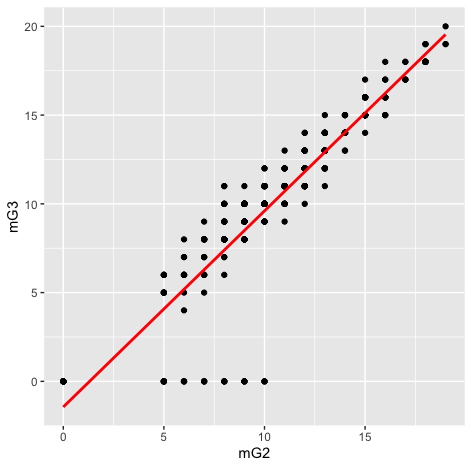
> stats::cor.test(s_perform$mG2, s_perform$mG3, method='pearson')

Pearson's product-moment correlation

data:  s_perform$mG2 and s_perform$mG3
t = 40.977, df = 380, p-value < 2.2e-16
alternative hypothesis: true correlation is
not equal to 0
95 percent confidence interval:
0.8826652 0.9200050
sample estimates:
cor 
0.9030267 
                                  
                              
```
Result:
We can observe from the graph that there is a strong positive linear correlation, which implies we have satisfied our assumptions for pearson test they are:
From Pearson correlation,we get a correlation of 0.90, which means the effect size is large(Acc. to cohen's effect size heuristic). Assuming our alpha level = 0.05, our p-value(0.001) < 0.05 => The correlation is statistically signigficant. And so we have evidence to reject null hypothesis in favor of the alternate which is there is a relationship between mG2 and mG3

Report for Research Question 1:

The relationship between mG3(Final math grade achieved by students) and mG2(math grade achieved in Grade 2) was investigated using a Pearson correlation. A strong positive correlation was found(r=0.90,n=380,p< 0.001).
Question:2 Is there significant difference in the mean of mG3 and students trying for higher education or not?

T-test: The t test tells you how significant the differences between groups are; In other words it lets you know if those differences (measured in means) could have happened by chance.

Assumptions of t-test:
- Normality: Since it is a parametric test, it depends on the normality of the variable.
- Homogeneity of variance: Variances in these populations are roughly equal.
Hypothesis (Two-tailed):
Null Hypothesis H0: There is no difference in mean mG3 score who try for higher studies and who do not try for higher studies
Alternate Hypothesis HA: There is a difference in mean mG3 score who try for higher studies and who do not try for higher studies
Code: #Getting descriptive stastitics by group - output as a matrix psych::describeBy(s_perform$mG3, s_perform$higher.m, mat=TRUE) #Levene's test car::leveneTest(mG3 ~ higher.m, data=s_perform) #Pr(>F) is your probability - in this case it is not statistically significant so we can assume homogeneity #Conducting the t-test from package stats #In this case we can use the var.equal = TRUE option to specify equal variances and a pooled variance estimate stats::t.test(mG3 ~ higher.m,var.equal=TRUE,data=s_perform) #Statistically significant difference was found res <- stats::t.test(mG3 ~ higher.m,var.equal=TRUE,data=s_perform) #Calculating Cohen's d #Using function from effectsize package effectsize::t_to_d(t = res$statistic, res$parameter) #Eta squared calculation effes=round((res$statistic*res$statistic)/ ((res$statistic*res$statistic)+(res$parameter)),3) effes
Output: > psych::describeBy(s_perform$mG3, s_perform$higher.m, mat=TRUE) item group1 vars n mean sd median trimmed mad min max range skew kurtosis se X11 1 no 1 18 5.50000 4.643148 8 5.43750 2.9652 0 12 12 -0.2580732 -1.8187883 1.0944005 X12 2 yes 1 364 10.62912 4.561466 11 11.03767 4.4478 0 20 20 -0.7262715 0.4110525 0.2390858 > car::leveneTest(mG3 ~ higher.m, data=s_perform) Levene's Test for Homogeneity of Variance (center = median) Df F value Pr(>F) group 1 0.356 0.5511 380 > stats::t.test(mG3 ~ higher.m,var.equal=TRUE,data=s_perform) Two Sample t-test data: mG3 by higher.m t = -4.6531, df = 380, p-value = 4.523e-06 alternative hypothesis: true difference in means is not equal to 0 95 percent confidence interval: -7.296493 -2.961749 sample estimates: mean in group no mean in group yes 5.50000 10.62912 > effectsize::t_to_d(t = res$statistic, res$parameter) d | 1e+02% CI ---------------------- -0.48 | [-0.68, -0.27] > effes t 0.054
Result:
Report for Research Question 2:

"An independent-samples t-test was conducted to compare the mean scores of mG3 for students who are trying for higher education and those who do not. A significant difference in the scores for mG3 was found ( M=10.63, SD= 4.56 for students who are trying for higher studies , M= 5.50,SD= 4.64 for students who are not trying for higher studies),(t(380)= -4.65, p = 0.01). A medium effect size was also indicated by Cohen's d value (-0.48)."

Question:3 Is there a Relationship between mG3 and their study-time?

Group: 1 - < 2 hours, Group: 2 - 2 to 5 hours, Group: 3 - 5 to 10 hours, or Group: 4 - >10 hours

ANOVA is an Omnibus test

It test for an overall difference between groups.
It tells us that the group means are different.
It doesn’t tell us exactly which means differ-We need to conduct post-hoc tests (additional tests after the ANOVA) to find out where the differences lie

Assumptions of ANOVA-test:

Normality: Since it is a parametric test, it depends on the normality of the variable.
Homogeneity of variance: Variances in these populations are roughly equal.

Null Hypothesis: The means of different groups of study-time are same.
Alternate Hypothesis: The means of different groups of study-time are different

Code:


                                #Get descriptive stastitics by group - output as a matrix
psych::describeBy(s_perform$mG3, s_perform$studytime.m, mat=TRUE)

#Conducting Bartlett's test for homogeneity of variance in librarycar
stats::bartlett.test(mG3~ studytime.m, data=s_perform)

#In this case we can use Tukey as the post-hoc test option since variances in the groups are equal 
userfriendlyscience::oneway(as.factor(s_perform$studytime.m),
y=s_perform$mG3,posthoc='Tukey')


#use the aov function - same as one way but makes it easier to 
access values for reporting
res2<-stats::aov(mG3~ studytime.m, data=s_perform)

#Get the F statistic into a variable to make reporting easier
fstat<-summary(res2)[[1]][["F value"]][[1]]

#Get the p value into a variable to make reporting easier
aovpvalue<-summary(res2)[[1]][["Pr(>F)"]][[1]]

#Calculate effect
aoveta<-sjstats::eta_sq(res2)[2]

Output:


                            > psych::describeBy(s_perform$mG3, s_perform$studytime.m, mat=TRUE)
item group1 vars   n     mean       sd median  trimmed    mad min max range       skew    kurtosis        se
X11    1      1    1 103 10.09709 4.991197   10.0 10.40964 4.4478   0  19    19 -0.6252929 -0.14768278 0.4917973
X12    2      2    1 190 10.10000 4.358960   10.0 10.50000 2.9652   0  19    19 -0.7165936  0.39850037 0.3162322
X13    3      3    1  62 11.37097 4.805168   11.5 11.92000 3.7065   0  19    19 -0.9149251  0.58114988 0.6102569
X14    4      4    1  27 11.25926 5.281263   12.0 11.56522 4.4478   0  20    20 -0.6998656 -0.07392943 1.0163795
                            
                            > stats::bartlett.test(mG3~ studytime.m, data=s_perform)

Bartlett test of homogeneity of variances

data:  mG3 by studytime.m
Bartlett's K-squared = 3.5886, df = 3, p-value = 0.3095
                            
                            > userfriendlyscience::oneway(as.factor(s_perform$studytime.m),y=s_perform$mG3,posthoc='Tukey')
### Oneway Anova for y=mG3 and x=studytime.m (groups: 1, 2, 3, 4)

Omega squared: 95% CI = [NA; .04], point estimate = 0
Eta Squared: 95% CI = [0; .03], point estimate = .01

                                    SS  Df    MS   F    p
Between groups (error + effect)  104.88   3 34.96 1.6 .189
Within groups (error only)      8265.78 378 21.87         


### Post hoc test: Tukey

diff  lwr   upr  p adj
2-1 0     -1.47 1.48 1.000
3-1 1.27  -0.67 3.21 .328 
4-1 1.16  -1.45 3.77 .659 
3-2 1.27  -0.49 3.04 .248 
4-2 1.16  -1.32 3.64 .624 
4-3 -0.11 -2.89 2.67 1.000

> aoveta
  etasq
 0.008

Result:


                                        Bartlett’s test : For homogeneity of variance
                                            

                                                
Null Hypothesis: All variances are equal. 
                                               
 Alternate Hypothesis: All variances are not equal.
                                                
 From the test, we can see p-value is 0.31,which is greater than 0.05,
                                                so it is not statistically significant, thus accepting null hypothesis(Homogenity).
                                        
                                        

                                        
                                            
                                            The p-value of the ANOVA-test(0.19) > 0.05, so we accept the null hypothesis
                                            of equal means among groups and reject the alternate hypothesis of different means
                                            among groups. 
                                            
No Statistically significant difference was found.
                                        
                                        

                                        
                                            Eta squared: 
                                            
                                                eta squared = sum of squares between groups/total sum of squares (from our ANOVA output (rounded up))

Report for Research Question 3:

A one-way between groups analysis of Variance(Anova) was conducted to explore the impact of study-time of a student on mG3. study-time variable was divided in to 4 groups( Group: 1 - < 2 hours, Group: 2 - 2 to 5 hours, Group: 3 - 5 to 10 hours, or Group: 4 - >10 hours). There was not statistically significant difference in the mG3 scores, p>0.05, which is also statistically insignificant .The effect size was calculated using eta-squared was (0.08) which is small.

Question:4 Is there a difference between students with different family size(less than 3 and greater than 3) in terms of whether they get family support?

Null Hypothesis: There is no difference between students with different family size(less than 3 and greater than 3) in terms of whether they get family support
Alternate Hypothesis:There is difference between students with different family size(less than 3 and greater than 3) in terms of whether they get family support

Chi-square Test:

The same variable is measured for each sample by classifying individual subjects into categories of the variable.
The data are presented in a matrix with the different samples defining the rows and the categories of the variable defining the columns.
The data, called observed frequencies, simply show how many individuals from the sample are in each cell of the matrix.

Code:


                                #Use the Crosstable function
#CrossTable(predictor, outcome, fisher = TRUE, chisq = TRUE,expected = TRUE)
gmodels::CrossTable(s_perform$famsize, s_perform$famsup.m,fisher = TRUE, chisq = TRUE, expected = TRUE, sresid = TRUE,format = "SPSS")


#Create your contingency table
mytable<-xtabs(~famsup.m+famsize, data=s_perform)

ctest<-stats::chisq.test(mytable, correct=TRUE)#chi square test
#correct=TRUE to get Yates correction needed for 2x2 table

ctest#will give you the details of the test statistic and p-value
ctest$expected#expected frequencies
ctest$observed#observed frequencies
ctest$p.value

#Calculate effect size
sjstats::phi(mytable)
sjstats::cramer(mytable)

Output:


                            > gmodels::CrossTable(s_perform$famsize, s_perform$famsup.m, fisher = TRUE, chisq = TRUE, expected = TRUE, sresid = TRUE, format = "SPSS")

Cell Contents
|-------------------------|
|                   Count |
|         Expected Values |
| Chi-square contribution |
|             Row Percent |
|          Column Percent |
|           Total Percent |
|            Std Residual |
|-------------------------|

Total Observations in Table:  382 

                | s_perform$famsup.m 
s_perform$famsize |       no  |      yes  | Row Total | 
------------------|-----------|-----------|-----------|
            GT3 |       97  |      181  |      278  | 
                |  104.796  |  173.204  |           | 
                |    0.580  |    0.351  |           | 
                |   34.892% |   65.108% |   72.775% | 
                |   67.361% |   76.050% |           | 
                |   25.393% |   47.382% |           | 
                |   -0.762  |    0.592  |           | 
------------------|-----------|-----------|-----------|
            LE3 |       47  |       57  |      104  | 
                |   39.204  |   64.796  |           | 
                |    1.550  |    0.938  |           | 
                |   45.192% |   54.808% |   27.225% | 
                |   32.639% |   23.950% |           | 
                |   12.304% |   14.921% |           | 
                |    1.245  |   -0.968  |           | 
------------------|-----------|-----------|-----------|
    Column Total |      144  |      238  |      382  | 
                |   37.696% |   62.304% |           | 
------------------|-----------|-----------|-----------|


Statistics for All Table Factors


Pearson's Chi-squared test 
------------------------------------------------------------
Chi^2 =  3.418969     d.f. =  1     p =  0.06445125 

Pearson's Chi-squared test with Yates' continuity correction 
------------------------------------------------------------
Chi^2 =  2.994468     d.f. =  1     p =  0.08354934 


Fisher's Exact Test for Count Data
------------------------------------------------------------
Sample estimate odds ratio:  0.6507166 

Alternative hypothesis: true odds ratio is not equal to 1
p =  0.07526814 
95% confidence interval:  0.4011554 1.057151 

Alternative hypothesis: true odds ratio is less than 1
p =  0.04240359 
95% confidence interval:  0 0.9817213 

Alternative hypothesis: true odds ratio is greater than 1
p =  0.9748774 
95% confidence interval:  0.4317107 Inf 


    Minimum expected frequency: 39.20419 
                        
                            > ctest#will give you the details of the test statistic and p-value

Pearson's Chi-squared test with Yates' continuity correction

data:  mytable
X-squared = 2.9945, df = 1, p-value = 0.08355
                            
                            > ctest$expected#expected frequencies
            famsize
famsup.m      GT3      LE3
        no  104.7958 39.20419
        yes 173.2042 64.79581
                            
                            > ctest$observed#observed frequencies
        famsize
famsup.m GT3 LE3
     no   97  47
     yes 181  57
                            
                            ctest$p.value
[1] 0.08354934

Result:


                                        
                                            For one degree of freedom
                                               
 The critical value associated with p = 0.05 for Chi Square is 3.84 
                                                
 The critical value associated with p =0.01 it is 6.64
                                                Chi-square values higher than this critical value are associated with a statistically low probability that H0 holds.
                                                
                                                
                                                    In our case x² = 3 which is less than 3.84(critical value), Therefore
                                                    there is no significant association between family size and 
                                                    their support to the student

Report for Research Question 4

A Chi-Square test for independence (with Yates’ Continuity Correction) indicated no significant association between students's family size and getting family support, χ2(1,n=380)=2.99,p=0.05, phi=0.084).

Descriptive Statistics

Dispersion/Vairability

Exploring & Analysing the dataset

Assesing Normality for the continous variables mG2,mG3:

For mg3

Reporting Normality for mG2:

For mg3

Reporting Normality for mG3:

Correlation:

Research Questions:

Report for Research Question 1:

Report for Research Question 2:

Report for Research Question 3:

Report for Research Question 4