Model

Linear Regression:

It's a hypothetical model of the relationship between two variables.Here the model is linear
The two variables involved in this are called the Predictor(independent) and the response(dependent) variable.

Correlation:
It is used to assert the relationship between the variables, it could be strong/weak and positive/negative correlation.So we can describe the relationship with a straight line
Differential effect:
This test involves ANOVA and T-test, they are used to show the effect among different groups in the variable.
Normally distributed response variable.

Fit of the model: We use fitness of a model to show how good a model is in associating the variables.

Total Sum of Squares(SS _T ):It is the sum of the squares of the difference of each data point from the mean of the outcome variable.
Residual Sum of squares(SS _R): It is the distance between each data point and the regression line
SS_M Difference between the two is the amount of variation accounted for by the model. This gives the Model variability.
Residuals:It is the distance between the predicted value and the observed value.

Analysing the Regression Model:

R ²:

The R² is the proportion of variance in the outcome (response) variable which can be explained by the predictor (independent) variables. This gives the usefulness of the model.
An R² of 1 means the independent variable explains 100% of the variance in the dependent variable. Conversely 0 means it explains none.

R ² vs Adjusted R ²

Every time we add a predictor to a model, the R-squared increases, even if due to chance alone. It never decreases. Therefore, a model with more terms may appear to have a better fit simply because it has more terms.
If a model has too many predictors it begins to model the random noise in the data. This condition is known as overfitting the model and it produces misleadingly high R-squared values and a lessened ability to make predictions. Adjusted R²
Adjusts value of R² based on number of variables in the model. Adjusted R² is reported for multiple linear regression

Analysis of Variance(ANOVA):

It shows whether the regression model is better at predicting the response variable than using the mean.

Beta Values:

It gives the unit change of the response value with respect to the predictor value.
Standardized Beta Values:Gives the value in terms of standard deviation.Useful in case of comparing models.

Linear Regression equation:

Equation: y= b ₀+ b ₁X

where, b ₀ is the intercept and b ₁ is the regression coefficent.
Coefficients:

Coefficients gives the values to construct the linear equation(i.e. The intecept and the regression coefficent)

Standardized Coefficients:

These are used to find the standardised scores of the coefficients, which can be used to compare different models.

Multiple Linear Regression:

The relationship is described using a variation of the equation of a straight line.

Equation: y= b ₀+ b ₁X ₁+b ₂X ₂+b ₃X ₃

where, b1 to bn are the regression coefficient for variable 1 to n

Dummy Variables:

Categorical variables are hard to predict because they do not have any scale and it would be impossible to associate the change of it like a continous variable.
So we transform the categorical variable into a series of dummy variables which indicate whether a particular case has that particular characteristic. They are also called as indicator variables.

0 (reference category) and 1 (category of interest)
We can explore the differential effect for the category of interest when compared to the reference category
For 'p' different categories there should be (p-1) indicator variables.

Research Question 5:

Null Hypothesis:

Alternate Hypothesis:

Models:

Model 1:Comparing the relationship between mG2 and mG3:

Code:


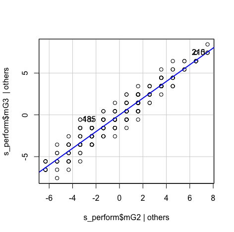
                                #Model1
scatter <- ggplot(s_perform, aes(s_perform$mG2, s_perform$mG3))
#Add a regression line
scatter + geom_point() + geom_smooth(method = "lm", colour = "Red", se = F) + labs(x = "mG2", y = "mG3") 


#Pearson Correlation
stats::cor.test(s_perform$mG2, s_perform$mG3, method='pearson')

#Building linear model using mG1,mG2 as predictors and mG3 as the dependent variable
s_perform$mG3<-na_if(s_perform$mG3,0)
model1<-lm(s_perform$mG3~s_perform$mG2)
anova(model1)
summary(model1)
lm.beta::lm.beta(model1)
stargazer(model1, type="text") #Tidy output of all the required stats

Result:

The p-value indicates our model is significant, so we can reject the null hypothesis and accept the alternate hypothesis(We can predict the values of mG3 with predictor variable mG2)
Increase marks in mG2 appears to associated with increase marks in mG3
There appears to be a strong positvie correlation bewteen the two
Therefore there is good justification for using regression to look at prediction.
The F statistic looks at whether the model as whole is statistically significant
In our case r ² value is 0.9348, which means around 93.5% of the variance mG3 can be explained by mG2.
Our linear regression model is Predicted mG3 = 0.32 + 0.99 * 'mG2'
In our case using the standardised coefficents our model equation becomes: Predicted mG3 = 0 + 0.97 * 'mG2'

Output:


                                > anova(model1)
Analysis of Variance Table

Response: s_perform$mG3
                Df Sum Sq Mean Sq F value    Pr(>F)    
s_perform$mG2   1 3444.5  3444.5  4902.1 < 2.2e-16 ***
Residuals     341  239.6     0.7                      
---
Signif. codes:  0 ‘***’ 0.001 ‘**’ 0.01 ‘*’ 0.05 ‘.’ 0.1 ‘ ’ 1
> summary(model1)

Call:
lm(formula = s_perform$mG3 ~ s_perform$mG2)

Residuals:
    Min      1Q  Median      3Q     Max 
-2.2447 -0.2199 -0.1579  0.7925  2.7801 

Coefficients:
                Estimate Std. Error t value Pr(>|t|)    
(Intercept)    0.31921    0.16692   1.912   0.0567 .  
s_perform$mG2  0.98759    0.01411  70.015   < 2e-16 ***
---
Signif. codes:  0 ‘***’ 0.001 ‘**’ 0.01 ‘*’ 0.05 ‘.’ 0.1 ‘ ’ 1

Residual standard error: 0.8382 on 341 degrees of freedom
    (39 observations deleted due to missingness)
Multiple R-squared:  0.935,	Adjusted R-squared:  0.9348 
F-statistic:  4902 on 1 and 341 DF,  p-value: < 2.2e-16

> lm.beta::lm.beta(model1)

Call:
lm(formula = s_perform$mG3 ~ s_perform$mG2)

Standardized Coefficients::
    (Intercept) s_perform$mG2 
    0.0000000     0.9669345 

> stargazer(model1, type="text") #Tidy output of all the required stats

===============================================
                        Dependent variable:    
                    ---------------------------
                                mG3            
-----------------------------------------------
mG2                          0.988***          
                                (0.014)          
                                                
Constant                      0.319*           
                                (0.167)          
                                                
-----------------------------------------------
Observations                    343            
R2                             0.935           
Adjusted R2                    0.935           
Residual Std. Error      0.838 (df = 341)      
F Statistic         4,902.121*** (df = 1; 341) 
===============================================
Note:               *p< 0.1; **p< 0.05; ***p< 0.01

Checking Assumptions:


                            
                                Outliers:
                            cooksd<-sort(cooks.distance(model1))
# plot Cook's distance
plot(cooksd, pch="*", cex=2, main="Influential Obs by Cooks distance")  
abline(h = 4*mean(cooksd, na.rm=T), col="red")  # add cutoff line
text(x=1:length(cooksd)+1, y=cooksd, labels=ifelse(cooksd>4*mean(cooksd, na.rm=T),names(cooksd),""), col="red")  # add labels

#finding rows related to influential observations
influential <- as.numeric(names(cooksd)[(cooksd > 4*mean(cooksd, na.rm=T))])  # influential row numbers
influential
stem(influential)
head(s_perform[influential, ])  # influential observations.
head(s_perform[influential, ]$mG1)  # influential observations - look at the values of mG1
head(s_perform[influential, ]$mG3)  # influential observations - look at the values of mG3

car::outlierTest(model1) # Bonferonni p-value for most extreme obs - Are there any cases where the outcome variable has an unusual variable for its predictor values?

                            
                                
                                Leverage:
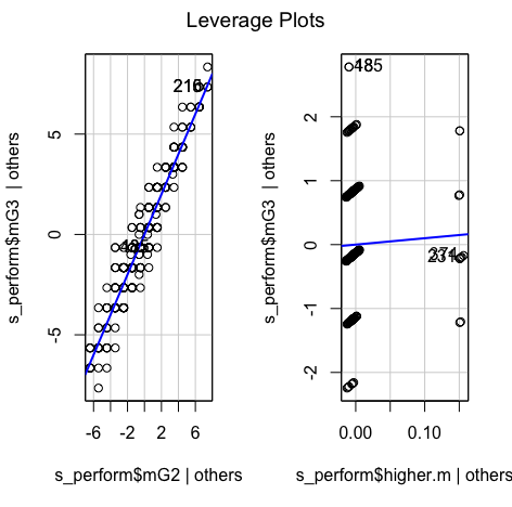
                                    car::leveragePlots(model1) # leverage plots
                                    
                                
                                Homocedasticity:
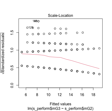
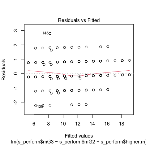
                                    #Assess homocedasticity 
plot(model1,1)
plot(model1, 3)
                                    
                                
                                Residuals:
                                    #Create histogram and  density plot of the residuals
plot(density(resid(model1))) 

#Create a QQ plotqqPlot(model, main="QQ Plot") #qq plot for studentized resid 
car::qqPlot(model1, main="QQ Plot") #qq plot for studentized resid

Output:


                                > influential
[1] 246  56   2  35 145 287 288 351 170 105  34 216 334 252  48 185 129
> stem(influential)

The decimal point is 2 digit(s) to the right of the |

0 | 03456
1 | 13579
2 | 25599
3 | 35

> head(s_perform[influential, ])  # influential observations.
# A tibble: 6 x 57
school sex     age address famsize Pstatus  Medu  Fedu Mjob  Fjob  reason nursery internet guardian.m traveltime.m
                                       
1 GP     M        16 U       GT3     T           4     3 heal… serv… reput… yes     yes      mother                1
2 GP     F        16 U       GT3     T           2     2 serv… other reput… no      yes      mother                2
3 GP     F        15 R       GT3     T           1     1 other other reput… no      yes      mother                1
4 GP     F        15 U       LE3     T           1     1 at_h… other other  yes     yes      mother                1
5 GP     F        18 R       GT3     T           1     1 at_h… other course no      no       mother                3
6 GP     M        17 U       GT3     T           2     1 other other home   yes     yes      mother                2
# … with 42 more variables: studytime.m , failures.m , schoolsup.m , famsup.m , paid.m ,
#   activities.m , higher.m , romantic.m , famrel.m , freetime.m , goout.m , Dalc.m ,
#   Walc.m , health.m , absences.m , mG1 , mG2 , mG3 , guardian.p , traveltime.p ,
#   studytime.p , failures.p , schoolsup.p , famsup.p , paid.p , activities.p ,
#   higher.p , romantic.p , famrel.p , freetime.p , goout.p , Dalc.p , Walc.p ,
#   health.p , absences.p , pG1 , pG2 , pG3 , intmark , Sex_num , inthighmG2 ,
#   inthigher.m 
> head(s_perform[influential, ]$mG1)  # influential observations - look at the values of mG1
[1] 19 13  8  7  9  8
> head(s_perform[influential, ]$mG3)  # influential observations - look at the values of mG3
[1] 20 11  5 10 10 10
> car::outlierTest(model1) # Bonferonni p-value for most extreme obs - Are there any cases where the outcome variable has an unusual variable for its predictor values?
No Studentized residuals with Bonferroni p < 0.05
Largest |rstudent|:
rstudent unadjusted p-value Bonferroni p
48 3.377184         0.00081718      0.28029
> car::qqPlot(model1, main="QQ Plot") #qq plot for studentized resid
[1]  48 185

Plots: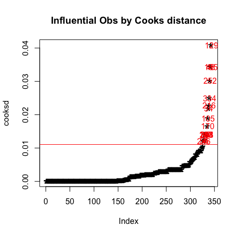

It can be observed that all the points are less than 1, So we don't have to worry about the outliers

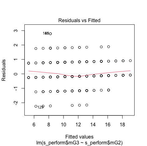
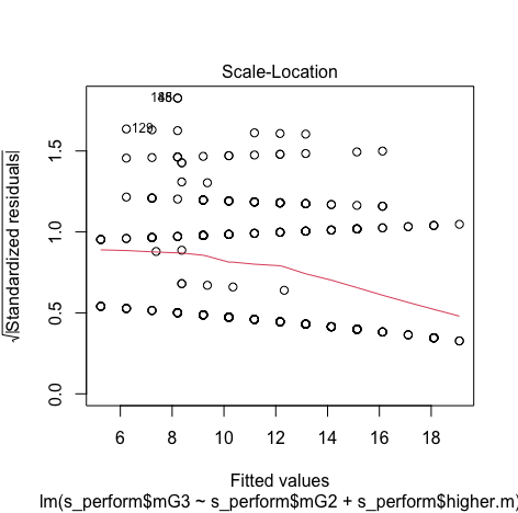
We can see that there is no pattern and points are equally distributed, therefore homoscedasticity is not an concern

Minimum and Maximum value is within the acceptable range(-3.29,+3.29) hence we do not have outliers.
Though the red lines are slightly distorted but this is not a huge problem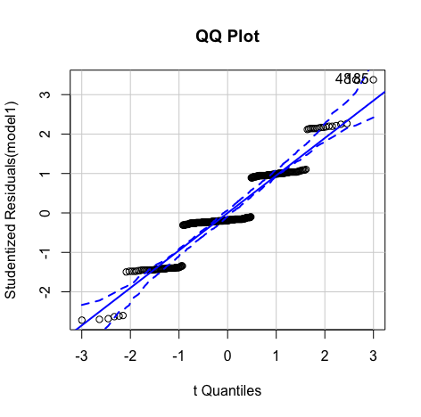

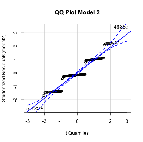
Errors are normally distributed

Model 2:Multiple Linear Regression(with mG2 and Higher as predictors and mG3 as dependent

We use the variable higher as a predictor, since it is a categorical type we use it as a dummy variable to understand the differential effect of the marks of students who are planning for higher studies and others.
Here, 0 (reference category, no) and 1 (category of interest, yes)

Code:


                                #Model2
model2<-lm(s_perform$mG3~s_perform$mG2+s_perform$higher.m)
anova(model2)
summary(model2)
stargazer(model2, type="text") #Tidy output of all the required stats
lm.beta(model2)
stargazer(model1, model2, type="text")

Result:

The p-value indicates our model is significant, so we can reject the null hypothesis and accept the alternate hypothesis(We can predict the values of mG3 with predictor variable mG2 and higher.m)
From the F-statistics and the p-value, our model is still significant.
New regression equation with higher.m as another predictor is: Predicted mG3 = 0.459 + 0.989 * 'mG2' - 0.161 * 'yes'
The new standardised reqression equation is: Predicted mG3 = 0 + 0.968 * 'mG2' - 0.009* 'yes'
when we calculate the equation for yes and no for higher studies: yes mG3 = 0+0.968-0.009=0.959
no mG3=0+0.968=0.968
We can see a small difference between the group yes and no.
We can see a slight change in the coefficent compared to model 1.
In this case the Adjusted R ² is 0.9347 which mean it could explain 93.5% of the variance of the mG3 from mG2.

Output:


                                > anova(model2)
Analysis of Variance Table

Response: s_perform$mG3
                    Df Sum Sq Mean Sq   F value Pr(>F)    
s_perform$mG2        1 3444.5  3444.5 4893.2132 < 2e-16 ***
s_perform$higher.m   1    0.3     0.3    0.3804 0.5378    
Residuals          340  239.3     0.7                     
---
Signif. codes:  0 ‘***’ 0.001 ‘**’ 0.01 ‘*’ 0.05 ‘.’ 0.1 ‘ ’ 1
> summary(model2)

Call:
lm(formula = s_perform$mG3 ~ s_perform$mG2 + s_perform$higher.m)

Residuals:
    Min      1Q  Median      3Q     Max 
-2.2322 -0.2101 -0.1549  0.8009  2.7899 

Coefficients:
                        Estimate Std. Error t value Pr(>|t|)    
(Intercept)            0.45893    0.28148   1.630    0.104    
s_perform$mG2          0.98897    0.01429  69.189   < 2e-16 ***
s_perform$higher.myes -0.16055    0.26033  -0.617    0.538    
---
Signif. codes:  0 ‘***’ 0.001 ‘**’ 0.01 ‘*’ 0.05 ‘.’ 0.1 ‘ ’ 1

Residual standard error: 0.839 on 340 degrees of freedom
    (39 observations deleted due to missingness)
Multiple R-squared:  0.935,	Adjusted R-squared:  0.9347 
F-statistic:  2447 on 2 and 340 DF,  p-value: < 2.2e-16

> stargazer(model2, type="text") #Tidy output of all the required stats

===============================================
                        Dependent variable:    
                    ---------------------------
                                mG3            
-----------------------------------------------
mG2                          0.989***          
                                (0.014)          
                                                
higher.myes                   -0.161           
                                (0.260)          
                                                
Constant                       0.459           
                                (0.281)          
                                                
-----------------------------------------------
Observations                    343            
R2                             0.935           
Adjusted R2                    0.935           
Residual Std. Error      0.839 (df = 340)      
F Statistic         2,446.797*** (df = 2; 340) 
===============================================
Note:               *p< 0.1; **p< 0.05; ***p< 0.01
> lm.beta(model2)

Call:
lm(formula = s_perform$mG3 ~ s_perform$mG2 + s_perform$higher.m)

Standardized Coefficients::
            (Intercept)         s_perform$mG2 s_perform$higher.myes 
            0.00000000            0.96828309           -0.00863115

Comparing Model 1 and Model 2:


                                > stargazer(model1, model2, type="text") 

=========================================================================
                                        Dependent variable:                 
                    -----------------------------------------------------
                                                mG3                         
                                (1)                        (2)            
-------------------------------------------------------------------------
mG2                          0.988***                   0.989***         
                                (0.014)                    (0.014)          
                                                                            
higher.myes                                              -0.161          
                                                        (0.260)          
                                                                            
Constant                      0.319*                     0.459           
                                (0.167)                    (0.281)          
                                                                            
-------------------------------------------------------------------------
Observations                   343                        343            
R2                            0.935                      0.935           
Adjusted R2                   0.935                      0.935           
Residual Std. Error      0.838 (df = 341)           0.839 (df = 340)     
F Statistic         4,902.121*** (df = 1; 341) 2,446.797*** (df = 2; 340)
=========================================================================
Note:                                         *p< 0.1; **p< 0.05; ***p< 0.01

Both the models are significant.
Adding the "higher" variable decreased the F-statistic of the model

Checking Assumptions:


                            
                                Outliers:
                            #Influential Outliers - Cook's distance
cooksd<-sort(cooks.distance(model2))
# plot Cook's distance
plot(cooksd, pch="*", cex=2, main="Influential Obs by Cooks distance")  
abline(h = 4*mean(cooksd, na.rm=T), col="red")  # add cutoff line
text(x=1:length(cooksd)+1, y=cooksd, labels=ifelse(cooksd>4*mean(cooksd, na.rm=T),names(cooksd),""), col="red")  # add labels

#find rows related to influential observations
influential <- as.numeric(names(cooksd)[(cooksd > 4*mean(cooksd, na.rm=T))])  # influential row numbers
stem(influential)
head(s_perform[influential, ])  # influential observations.
head(s_perform[influential, ]$mG2)  # influential observations - look at the values of mG2
head(s_perform[influential, ]$mG3)  # influential observations - look at the values of mG3
head(s_perform[influential, ]$higher.m)  # influential observations -look at the values of higher

car::outlierTest(model2) # Bonferonni p-value for most extreme obs - Are there any cases where the outcome variable has an unusual variable for its predictor values?   
                            
                                
                                Leverage:
                                    car::leveragePlots(model2) # leverage plots
                                    
                                
                                Homocedasticity:
                                    #Assess homocedasticity 
plot(model2,1)
plot(model2, 3)
                                    
                                
                                Residuals:
                                    #Create histogram and  density plot of the residuals
plot(density(resid(model2))) 

#Create a QQ plotqqPlot(model, main="QQ Plot") #qq plot for studentized resid 
car::qqPlot(model2, main="QQ Plot") #qq plot for studentized resid
                                    

                                
                                Collinearity:
                                    #Collinearity
vifmodel<-car::vif(model2)
vifmodel
#Tolerance
1/vifmodel

Output:


                                > head(s_perform[influential, ])  # influential observations.
# A tibble: 6 x 57
    school sex     age address famsize Pstatus  Medu  Fedu Mjob  Fjob  reason nursery internet guardian.m traveltime.m
                                           
1 GP     M        15 U       LE3     T           4     3 teac… serv… home   yes     yes      mother                1
2 GP     F        15 U       LE3     A           4     3 other other course yes     yes      mother                1
3 GP     M        18 U       LE3     T           3     3 serv… heal… home   yes     yes      father                1
4 MS     M        18 U       LE3     T           1     3 at_h… serv… course yes     yes      mother                1
5 GP     F        19 U       GT3     T           0     1 at_h… other course no      no       other                 1
6 GP     M        16 U       GT3     T           4     4 serv… serv… other  yes     yes      mother                1
# … with 42 more variables: studytime.m , failures.m , schoolsup.m , famsup.m , paid.m ,
#   activities.m , higher.m , romantic.m , famrel.m , freetime.m , goout.m , Dalc.m ,
#   Walc.m , health.m , absences.m , mG1 , mG2 , mG3 , guardian.p , traveltime.p ,
#   studytime.p , failures.p , schoolsup.p , famsup.p , paid.p , activities.p ,
#   higher.p , romantic.p , famrel.p , freetime.p , goout.p , Dalc.p , Walc.p ,
#   health.p , absences.p , pG1 , pG2 , pG3 , intmark , Sex_num , inthighmG2 ,
#   inthigher.m 
> head(s_perform[influential, ]$mG2)  # influential observations - look at the values of mG2
[1] 16  8  6  7  8  7
> head(s_perform[influential, ]$mG3)  # influential observations - look at the values of mG3
[1] 18  6  8  8  9  5
> head(s_perform[influential, ]$higher.m)  # influential observations -look at the values of higher
[1] "yes" "yes" "yes" "no"  "no"  "yes"
> car::outlierTest(model2) # Bonferonni p-value for most extreme obs - Are there any cases where the outcome variable has an unusual variable for its predictor values?
No Studentized residuals with Bonferroni p < 0.05
Largest |rstudent|:
    rstudent unadjusted p-value Bonferroni p
48 3.387117         0.00078934      0.27075
> car::leveragePlots(model2) # leverage plots

> #A density plot of the residuals
> plot(density(resid(model2))) 
> #Create a QQ plot qPlot(model, main="QQ Plot") #qq plot for studentized resid 
> car::qqPlot(model2, main="QQ Plot Model 2") #qq plot for studentized resid
[1]  48 185
> #Collinearity
> vifmodel<-car::vif(model2)
> vifmodel
        s_perform$mG2 s_perform$higher.m 
            1.025022           1.025022 
#Tolerance
> 1/vifmodel
s_perform$mG2 s_perform$higher.m 
    0.9755884          0.9755884

We can observe that the VIF values are less than 2.5 and 1/VIF values are greater than 0.4 . So we do not have multicollinearity problem.

Plots: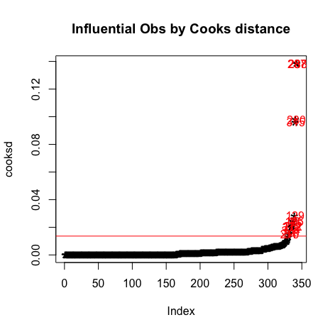

It can be observed that all the points are less than 1, So we don't have to worry about the outliers

We can see that there is no pattern and points are equally distributed, therefore homoscedasticity is not an concern

Minimum and Maximum value is within the acceptable range(-3.29,+3.29) hence we do not have outliers.
Though the red lines are slightly distorted but this is not a huge problem

Errors are normally distributed

Reporting Multiple linear Regression(Model 2):

Multiple regression analysis was conducted to determine the student's final math grade(mG3).. Marks obtained in second grade(mG2),going for higher studies(higher) were used as predictor variables. In order to include the higher education in the regression model it was recorded dummy variable higher_edu (0 for no, 1 for yes).Examination of the histogram, normal P-P plot of standardised residuals and the scatterplot of the dependent variable, academic satisfaction, and standardised residuals showed that the some outliers existed. However, examination of the standardised residuals showed that none could be considered to have undue influence (95% within limits of -1.96 to plus 1.96 and none with Cook’s distance >1 as outlined in Field (2013). Examination for multicollinearity showed that the tolerance and variance influence factor measures were within acceptable levels (tolerance >0.4, VIF < 2.5 ) as outlined in Tarling (2008). The scatterplot of standardised residuals showed that the data met the assumptions of homogeneity of variance and linearity. The data also meets the assumption of non-zero variances of the predictors.

Model 3:Multiple Linear Regression(with mG2 and Higher*mG2 as predictors and mG3 as dependent variable.

Model 2 was fine but it does assume that the gap in mG3 marks between students trying for higher studies and others remains constant (at 0.170 points) regardless of a student’s prior mG2 marks.
But it may be that high achieving students who are not trying for higher studies at mG2 could be outperforming students who are trying for higher studies at mG3 and/or that low performing students trying for higher studies at mG2 may fall even further behind their students who are not trying for higher studies at mG3?
We are hypothesising here, in effect, that the gradients of both these lines of best fit might not be the same and thus these two lines might not actually be parallel.
We can test this hypothesis by adding what is referred to as an ‘interaction term’ to the model that is basically a new variable calculated by multiplying Higher’ by ‘mG2’.

Code:


                                #Model 3
#interaction effect
#create interaction term - adding a new variable to the dataset inthighmG2
s_perform$inthigher.m <- ifelse(s_perform$higher.m=='yes',1,0)
s_perform$inthigher.m
s_perform$inthighmG2<-as.numeric(s_perform$inthigher.m)*s_perform$mG2
s_perform$inthighmG2
model3 <-lm(s_perform$mG3~s_perform$mG2+s_perform$higher.m+s_perform$inthighmG2)
anova(model3)
summary(model3)
stargazer(model3, type="text") #Tidy output of all the required stats
lm.beta(model3)
stargazer(model2, model3, type="text")

Result:

The p-value indicates our model is significant, so we can reject the null hypothesis and accept the alternate hypothesis(We can predict the values of mG3 with predictor variable mG2, higher.m and indication term mG2*higher.m)
From the F-statistics and the p-value, our model is still significant.
New regression equation with higher.m as another predictor is: Predicted mG3 = 2.48 + 0.755 * 'mG2' -2.197 * 'yes' + 0.235 * 'yes*mG2'
The new standardised reqression equation is: Predicted mG3 = 0+ 0.739 * 'mG2' -0.118 * 'yes'+ 0.269 * 'yes*mG2'
when we calculate the equation for yes and no for higher studies with the interaction: yes mG3 = 0+0.739-0.118+0.269=0.89
no mG3=0+0.739+0.269=1.008
We can see how the inclusion of the interaction term has basically had the consequence of giving us two lines of best fit (one for yes and one for no) that now have differing intercepts as well as differing gradients or slopes.
On this occasion we already knew that the difference in the slopes was minor (and not statistically significant) and this is confirmed by these two lines of best fit where the difference in the gradients of both lines (0.739 compared to 0.968) is marginal and wouldn’t even be obvious to the eye if the two lines were plotted on a graph.
We would conclude that this interaction term has no significant effect on the model.
In this case the Adjusted R ² is 0.9347 which mean it could explain 93.5% of the variance of the mG3 from mG2.

Output:


                                > anova(model3)
Analysis of Variance Table

Response: s_perform$mG3
                        Df Sum Sq Mean Sq   F value Pr(>F)    
s_perform$mG2          1 3444.5  3444.5 4899.7341 < 2e-16 ***
s_perform$higher.m     1    0.3     0.3    0.3809 0.5375    
s_perform$inthighmG2   1    1.0     1.0    1.4531 0.2289    
Residuals            339  238.3     0.7                     
---
Signif. codes:  0 ‘***’ 0.001 ‘**’ 0.01 ‘*’ 0.05 ‘.’ 0.1 ‘ ’ 1
> summary(model3)

Call:
lm(formula = s_perform$mG3 ~ s_perform$mG2 + s_perform$higher.m + 
    s_perform$inthighmG2)

Residuals:
    Min      1Q  Median      3Q     Max 
-2.2252 -0.2057 -0.1569  0.8041  2.7943 

Coefficients:
                        Estimate Std. Error t value Pr(>|t|)    
(Intercept)             2.4804     1.7004   1.459 0.145565    
s_perform$mG2           0.7549     0.1947   3.877 0.000127 ***
s_perform$higher.myes  -2.1966     1.7089  -1.285 0.199549    
s_perform$inthighmG2    0.2353     0.1952   1.205 0.228872    
---
Signif. codes:  0 ‘***’ 0.001 ‘**’ 0.01 ‘*’ 0.05 ‘.’ 0.1 ‘ ’ 1

Residual standard error: 0.8385 on 339 degrees of freedom
    (39 observations deleted due to missingness)
Multiple R-squared:  0.9353,	Adjusted R-squared:  0.9347 
F-statistic:  1634 on 3 and 339 DF,  p-value: < 2.2e-16

> stargazer(model3, type="text") #Tidy output of all the required stats

===============================================
                        Dependent variable:    
                    ---------------------------
                                mG3            
-----------------------------------------------
mG2                          0.755***          
                                (0.195)          
                                                
higher.myes                   -2.197           
                                (1.709)          
                                                
inthighmG2                     0.235           
                                (0.195)          
                                                
Constant                       2.480           
                                (1.700)          
                                                
-----------------------------------------------
Observations                    343            
R2                             0.935           
Adjusted R2                    0.935           
Residual Std. Error      0.838 (df = 339)      
F Statistic         1,633.856*** (df = 3; 339) 
===============================================
Note:               *p< 0.1; **p< 0.05; ***p< 0.01
> lm.beta(model3)

Call:
lm(formula = s_perform$mG3 ~ s_perform$mG2 + s_perform$higher.m + 
    s_perform$inthighmG2)

Standardized Coefficients::
            (Intercept)         s_perform$mG2 s_perform$higher.myes  s_perform$inthighmG2 
            0.0000000             0.7391138            -0.1180848             0.2694700

Comparing Model 2 and Model 3:


                                > stargazer(model2, model3, type="text") 

=========================================================================
                                     Dependent variable:                 
                    -----------------------------------------------------
                                             mG3                         
                               (1)                        (2)            
-------------------------------------------------------------------------
mG2                          0.989***                   0.755***         
                             (0.014)                    (0.195)          
                                                                         
higher.myes                   -0.161                     -2.197          
                             (0.260)                    (1.709)          
                                                                         
inthighmG2                                               0.235           
                                                        (0.195)          
                                                                         
Constant                      0.459                      2.480           
                             (0.281)                    (1.700)          
                                                                         
-------------------------------------------------------------------------
Observations                   343                        343            
R2                            0.935                      0.935           
Adjusted R2                   0.935                      0.935           
Residual Std. Error      0.839 (df = 340)           0.838 (df = 339)     
F Statistic         2,446.797*** (df = 2; 340) 1,633.856*** (df = 3; 339)
=========================================================================
Note:                                         *p< 0.1; **p< 0.05; ***p< 0.01

Both the models are significant.
Adding the "higher" variable decreased the F-statistic of the model

Checking Assumptions:


                    
                        Outliers:
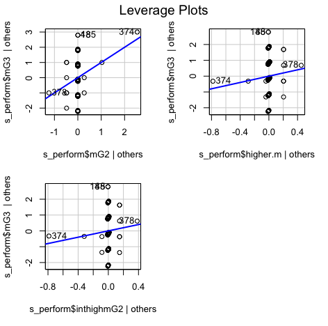
                    #Influential Outliers - Cook's distance
cooksd<-sort(cooks.distance(model3))
# plot Cook's distance
plot(cooksd, pch="*", cex=2, main="Influential Obs by Cooks distance")  
abline(h = 4*mean(cooksd, na.rm=T), col="red")  # add cutoff line
text(x=1:length(cooksd)+1, y=cooksd, labels=ifelse(cooksd>4*mean(cooksd, na.rm=T),names(cooksd),""), col="red")  # add labels

#find rows related to influential observations
influential <- as.numeric(names(cooksd)[(cooksd > 4*mean(cooksd, na.rm=T))])  # influential row numbers
stem(influential)
head(s_perform[influential, ])  # influential observations.
head(s_perform[influential, ]$mG2)  # influential observations - look at the values of mG2
head(s_perform[influential, ]$mG3)  # influential observations - look at the values of mG3
head(s_perform[influential, ]$higher.m)  # influential observations -look at the values of higher
head(s_perform[influential, ]$inthighmG2)  # influential observations -look at the values of interaction var
                    
                        
                        Leverage:
                            car::leveragePlots(model3) # leverage plots
                            
                        
                        Homocedasticity:
                            #Assess homocedasticity 
plot(model3,1)
plot(model3, 3)
                            
                        
                        Residuals:
                            #Create histogram and  density plot of the residuals
plot(density(resid(model3))) 

#Create a QQ plotqqPlot(model, main="QQ Plot") #qq plot for studentized resid 
car::qqPlot(model1, main="QQ Plot") #qq plot for studentized resid
                            
                        
                        Collinearity:
                            #Collinearity
vifmodel<-car::vif(model2)
vifmodel
#Tolerance
1/vifmodel

Results:


                        > head(s_perform[influential, ])  # influential observations.
# A tibble: 6 x 57
    school sex     age address famsize Pstatus  Medu  Fedu Mjob  Fjob  reason nursery internet guardian.m traveltime.m
                                           
1 GP     F        16 U       GT3     T           1     1 serv… serv… course no      yes      father                4
2 GP     M        15 U       GT3     T           2     2 serv… serv… course yes     yes      father                1
3 GP     F        17 U       GT3     T           4     3 other other reput… yes     yes      mother                1
4 GP     M        18 U       GT3     T           2     1 serv… serv… other  no      yes      mother                1
5 GP     M        17 U       GT3     T           2     1 other other home   yes     yes      mother                2
6 GP     M        17 U       GT3     T           2     1 other other home   yes     yes      mother                2
# … with 42 more variables: studytime.m , failures.m , schoolsup.m , famsup.m , paid.m ,
#   activities.m , higher.m , romantic.m , famrel.m , freetime.m , goout.m , Dalc.m ,
#   Walc.m , health.m , absences.m , mG1 , mG2 , mG3 , guardian.p , traveltime.p ,
#   studytime.p , failures.p , schoolsup.p , famsup.p , paid.p , activities.p ,
#   higher.p , romantic.p , famrel.p , freetime.p , goout.p , Dalc.p , Walc.p ,
#   health.p , absences.p , pG1 , pG2 , pG3 , intmark , Sex_num , inthighmG2 ,
#   inthigher.m 
> head(s_perform[influential, ]$mG2)  # influential observations - look at the values of mG2
[1] 8 8 6 9 8 8
> head(s_perform[influential, ]$mG3)  # influential observations - look at the values of mG3
[1] 11 11  4  8 10 10
> head(s_perform[influential, ]$higher.m)  # influential observations -look at the values of higher
[1] "yes" "yes" "yes" "no"  "no"  "no" 
> head(s_perform[influential, ]$inthighmG2)  # influential observations -look at the values of interaction var
[1] 8 8 6 0 0 0
> car::outlierTest(model3) # Bonferonni p-value for most extreme obs - Are there any cases where the outcome variable has an unusual variable for its predictor values?
No Studentized residuals with Bonferroni p < 0.05
Largest |rstudent|:
    rstudent unadjusted p-value Bonferroni p
48 3.395179         0.00076746      0.26324
> car::leveragePlots(model3) # leverage plots
> #Assess homocedasticity 
> plot(model3,1)
> plot(model3, 3)
> #A density plot of the residuals
> plot(density(resid(model3))) 
> #Create a QQ plot qPlot(model, main="QQ Plot") #qq plot for studentized resid 
> car::qqPlot(model3, main="QQ Plot Model 3") #qq plot for studentized resid
[1]  48 185

vifmodel
s_perform$mG2   s_perform$higher.m s_perform$inthighmG2 
    190.43212             44.23102            261.88128 
> #Tolerance
> 1/vifmodel
s_perform$mG2   s_perform$higher.m s_perform$inthighmG2 
  0.005251215          0.022608568          0.003818524

We can observe that the VIF values are greater than 2.5 and 1/VIF values are less than 0.4 . So we have multicollinearity problem.
After adding the interaction term we can observe multicollinearity in the model.

Plots: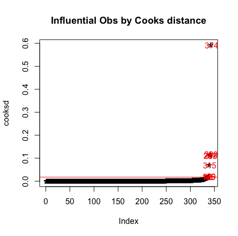

It can be observed that all the points are less than 1, So we don't have to worry about the outliers

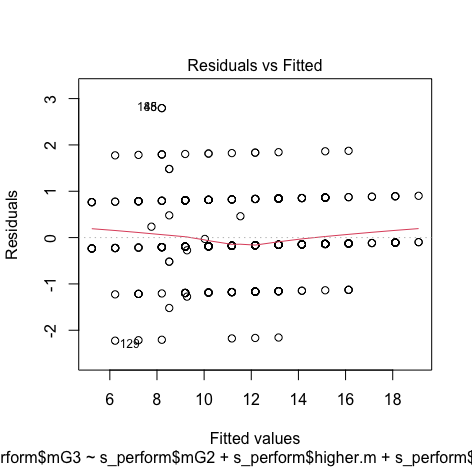
We can see that there is no pattern and points are equally distributed, therefore homoscedasticity is not an concern

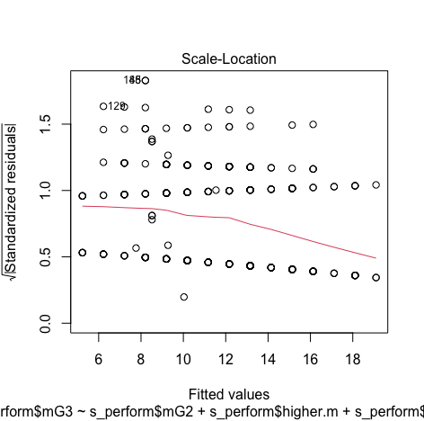
Minimum and Maximum value is within the acceptable range(-3.29,+3.29) hence we do not have outliers.
Though the red lines are slightly distorted but this is not a huge problem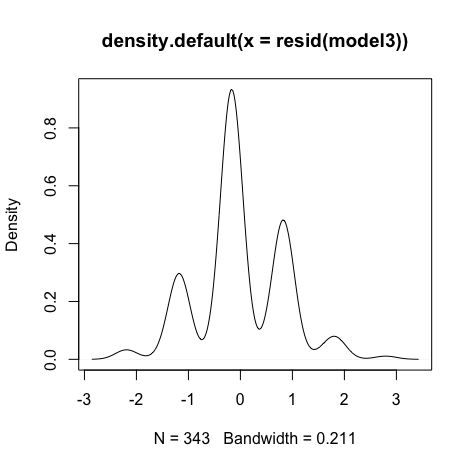

Errors are normally distributed

Reporting Multiple linear Regression(Model 3):

Multiple regression analysis was conducted to determine the student's final math grade(mG3).. Marks obtained in second grade(mG2),going for higher studies(higher) were used as predictor variables In order to include the higher education in the regression model it was recorded dummy variable higher_edu (0 for no, 1 for yes) and an interaction term was introduced by multiplying (inthigher * mG2) .Examination of the histogram, normal P-P plot of standardised residuals and the scatterplot of the dependent variable, academic satisfaction, and standardised residuals showed that the some outliers existed. However, examination of the standardised residuals showed that none could be considered to have undue influence (95% within limits of -1.96 to plus 1.96 and none with Cook’s distance >1 as outlined in Field (2013). Examination for multicollinearity showed that the tolerance and variance influence factor measures were outside acceptable levels (tolerance < 0.4, VIF > 2.5 ) as outlined in Tarling (2008).

Logistic Regression:

Unlike Linear Regression it does not predict the numerical value with given inputs rather it gives the probability of the given input value in a class or category.
It is used to predict the categorical(nominal) value using one or more categorical input or a continous input.
This is used because a categorical outcome variable violates the assumptions of linear regression.
It classifies each record based on their predictors into the category with highest probablity.
Assumptions: We assume that the input space can be divided into two regions(indicating the two categories) by a linear line(boundary). This is called linear-separable.
For two dimensions, this boundary is a straight line- no curving.
For three dimensions, its a plane. And so on.
Equation: b₀ + b₁x₁ + b₂x₂ where x₁ aand x₂ are the two predictor variables.
Mathematically, the higher the magnitude of this value, the greater is the distance between the point and the boundary.

Binary logistic Regression: The outcome variable is a dummy variable with two categories(0 or 1).
Odds = probability of an event occurring / probability of event not occurring (p/1-p)
There is no assumption of linearity between variables
It is however sensitive to high correlation between predictor variables (multicollinearity)
Indicates the change in odds resulting from a unit change in the predictor.
OR > 1: Predictor increases, Probability of outcome also increases .
OR < 1: Predictor increases, Probability of outcome decreases.
Omnibus test of model is used to check that the new model (with explanatory variables included) is an improvement over the baseline model.
It uses chi-square tests to see if there is a significant difference between the baseline model (null) and the model created
Deviance residuals, are a measure of model fit
AIC adjusts for increasing the number of parameters can be used to avoid overfitting.
Minimizing the AIC selects the model where the improvement in log likelihood is not worth the penalty for increasing the number of parameters. Used for comparing model.
Usefulness of a model: Cox and Snell R2 and Nagelkerke R² are pseudo R² statistics
Sensitivity vs Specificity
Sensitivity (also called the true positive rate, or the recall in some fields)
Sensitivity= true positives/(true positive + false negative)
It gives the percentage of the group with the characteristic of interest that has been accurately identified by the model
Specificity (also called the true negative rate)
Specificity=true negatives/(true negative + false positives)
It gives the percentage of the group not with the characteristic of interest that has been accurately identified by the model

ROC curve:

Used to see how any predictive model can distinguish between the true positives and negatives by plotting
sensitivity, the probability of predicting a real positive will be a positive, against 1-specificity, the probability of predicting a real negative will be a positive.
The ROC curve plots out the sensitivity and specificity for every possible decision rule cutoff between 0 and 1 for a model.
The further the curve is from the lower diagonal line, the better the model is at discriminating between positives and negatives in general.
AUC is the percentage of area under this curve.

Research Question 6:

Can we predict whether a student will go for higher studies(higher.m) with various predictors using logistic Regression ?

Model 1:

Code:


                                    #Make sure categorical data is used as factors

logmodel1 <- glm(as.factor(higher.m) ~ as.factor(sex), data = s_perform, na.action = na.exclude, family = binomial(link=logit))

#Full summary of the model
summary(logmodel1)

#Chi-square plus significance
lmtest::lrtest(logmodel1)


#Output the sensitivity, specificity, and ROC plot
Epi::ROC(form=as.factor(s_perform$higher.m) ~as.factor(s_perform$sex), plot="ROC")

#Pseudo Rsquared 
DescTools::PseudoR2(logmodel1, which="CoxSnell")
DescTools::PseudoR2(logmodel1, which="Nagelkerke")

#Summary of the model with co-efficients
stargazer(logmodel1, type="text")


#Exponentiate the co-efficients
exp(coefficients(logmodel1))
## odds ratios and 95% CI 
cbind(Estimate=round(coef(logmodel1),4),
        OR=round(exp(coef(logmodel1)),4))

#Probability of answering yes when male 
arm::invlogit(coef(logmodel1)[1]+ coef(logmodel1)[2]*0)#YES this is the same as just having the 1st co-efficient
#Probability of answering yes when female 
arm::invlogit(coef(logmodel1)[1]+ coef(logmodel1)[2]*1)

generalhoslem::logitgof(as.factor(s_perform$higher.m), fitted(logmodel1))

Result:

The Pr(>|z|) column shows the two-tailed p-values testing the null hypothesis that the coefficient is equal to zero (i.e. no significant effect).
The usual cut-off value is 0.05.
From this model it appears that gender does not have a significant effect on the log-odds ratio of the dependent variable.
The z statistic or Wald statistic is calculated to get the significance of the predictor.
The effect of the predictors negative.
When gender is male the expected change in the log odds is -1.76, a decrease in comparison to being female However we know this is statistically significant.
The intercept or constant are the odds of answering yes to planning for higher studies when male 65
The odds are higher when female in comparison to being male.
Predicted probability of answering yes when male is 97.95% Predicted probability of answering yes when female is 91.85 %
The Chi-square statistic is 10.08 df=-1, which is NOT statistically significant (p < 0.01)
AIC is 139.04
Between 2.60% and 8.24% of the variability of responses to whether students said they are going for higher studies or not
From the graph we can see the Sensitivity is 53.6% and the Specificity is 83.3%
The positive predictive value is the percentage of the cases the model classifies as having the characteristic that is actually observed in this group.(91.8%)
The negative predictive value is the percentage of the cases the model classifies as not having the characteristic that is actually observed in this group. (-1.5%)
From the graph, AUC is 0.685 (.5 is considered weak, 0.8 strong) so ours is moderate.

Plots:

Output:


                                    > summary(logmodel1)

Call:
glm(formula = as.factor(higher.m) ~ as.factor(sex), family = binomial(link = logit), 
    data = s_perform, na.action = na.exclude)

Deviance Residuals: 
    Min       1Q   Median       3Q      Max  
-2.8947   0.1747   0.1747   0.4124   0.4124  

Coefficients:
                Estimate Std. Error z value Pr(>|z|)    
(Intercept)       4.1744     0.5818   7.175 7.22e-13 ***
as.factor(sex)M  -1.7525     0.6411  -2.734  0.00627 ** 
---
Signif. codes:  0 ‘***’ 0.001 ‘**’ 0.01 ‘*’ 0.05 ‘.’ 0.1 ‘ ’ 1

(Dispersion parameter for binomial family taken to be 1)

    Null deviance: 145.12  on 381  degrees of freedom
Residual deviance: 135.04  on 380  degrees of freedom
AIC: 139.04

Number of Fisher Scoring iterations: 7

> #Chi-square plus significance
> lmtest::lrtest(logmodel1)
Likelihood ratio test

Model 1: as.factor(higher.m) ~ as.factor(sex)
Model 2: as.factor(higher.m) ~ 1
    #Df  LogLik Df  Chisq Pr(>Chisq)   
1   2 -67.521                        
2   1 -72.560 -1 10.079     0.0015 **
---
Signif. codes:  0 ‘***’ 0.001 ‘**’ 0.01 ‘*’ 0.05 ‘.’ 0.1 ‘ ’ 1
> #Output the sensitivity, specificity, and ROC plot
> Epi::ROC(form=as.factor(s_perform$higher.m) ~as.factor(s_perform$sex), plot="ROC")
> #Pseudo Rsquared 
> DescTools::PseudoR2(logmodel1, which="CoxSnell")
    CoxSnell 
0.0260388 
> DescTools::PseudoR2(logmodel1, which="Nagelkerke")
Nagelkerke 
0.08238383 
> #Summary of the model with co-efficients
> stargazer(logmodel1, type="text")

=============================================
                        Dependent variable:    
                    ---------------------------
                        as.factor(higher.m)    
---------------------------------------------
as.factor(sex)M            -1.753***         
                            (0.641)          
                                                
Constant                   4.174***          
                            (0.582)          
                                                
---------------------------------------------
Observations                  382            
Log Likelihood              -67.521          
Akaike Inf. Crit.           139.041          
=============================================
Note:             *p< 0.1; **p< 0.05; ***p< 0.01
> #Exponentiate the co-efficients
> exp(coefficients(logmodel1))
    (Intercept) as.factor(sex)M 
        65.0000000       0.1733333 
> ## odds ratios and 95% CI 
> cbind(Estimate=round(coef(logmodel1),4),
+       OR=round(exp(coef(logmodel1)),4))
                Estimate      OR
(Intercept)       4.1744 65.0000
as.factor(sex)M  -1.7525  0.1733
> #Probability of answering yes when male 
> arm::invlogit(coef(logmodel1)[1]+ coef(logmodel1)[2]*0)#YES this is the same as just having the 1st co-efficient
(Intercept) 
    0.9848485 
> #Probability of answering yes when female 
> arm::invlogit(coef(logmodel1)[1]+ coef(logmodel1)[2]*1)
(Intercept) 
    0.9184783 
> generalhoslem::logitgof(as.factor(s_perform$higher.m), fitted(logmodel1))

    Hosmer and Lemeshow test (binary model)

data:  as.factor(s_perform$higher.m), fitted(logmodel1)
X-squared = 4.4881e-27, df = -1, p-value = NA

Model 2:

Code:


                                    #Make sure categorical data is used as factors
            
logmodel2 <- glm(as.factor(higher.m) ~ as.factor(sex)+as.factor(romantic.m), data = s_perform, na.action = na.exclude, family = binomial(link=logit))


#Full summary of the model
summary(logmodel2)

#Chi-square plus significance
lmtest::lrtest(logmodel2)

#Pseudo Rsquared 
DescTools::PseudoR2(logmodel2, which="CoxSnell")
DescTools::PseudoR2(logmodel2, which="Nagelkerke")

#Output the sensitivity, specificity, and ROC plot
Epi::ROC(form=as.factor(s_perform$higher.m) ~as.factor(s_perform$sex)+as.factor(s_perform$romantic.m), plot="ROC")

#Summary of the model with co-efficients
stargazer(logmodel2, type="text")

#Exponentiate the co-efficients
exp(coefficients(logmodel2))
## odds ratios 
cbind(Estimate=round(coef(logmodel2),4),
      OR=round(exp(coef(logmodel2)),4))



#romantic.m 1 has a romantic relationship, 2 not having a romantic relationship
#1. Probability of answering yes when male and  having a relationship
arm::invlogit(coef(logmodel2)[1]+ coef(logmodel2)[2]*0)
#2. Probability of answering yes when female and having a relationship
arm::invlogit(coef(logmodel2)[1]+ coef(logmodel2)[2]*1)

#3.Probability of answering yes when male when not having a relationship
arm::invlogit(coef(logmodel2)[1]+ coef(logmodel2)[2]*0 +coef(logmodel2)[3]*0)
#4. Probability of answering yes when female when not having a relationship
arm::invlogit(coef(logmodel2)[1]+ coef(logmodel2)[2]*1 +coef(logmodel2)[3]*0)

Result:

Based on p-value, we can reject null hypothesis and accept alternate hypothesis
The Pr(>|z|) column shows the two-tailed p-values testing the null hypothesis that the coefficient is equal to zero (i.e. no significant effect).
The usual cut-off value is 0.05.
From this model it appears that gender and the romantic interest does not have a significant effect on the log-odds ratio of the dependent variable.
The z statistic or Wald statistic is calculated to get the significance of the predictor.
The effect of the predictors negative.
When gender is male the expected change in the log odds is -1.9, a decrease in comparison to being female and when the ßtudent is in a romantic relationship the log odds -1.47, a decreaase in comparison to not being in a romantic relationship.
However we know this is statistically significant.
The intercept or constant are the odds of answering yes to planning for higher studiies when female and not in a romantic interest 138.5
The odds are higher when male in comparison to being female and if they are not in a romantic relationship.
Predicted Probability of answering yes when male and having a relationship is 99.3% Predicted Probability of answering yes when female and having a relationship is 95.4% Predicted Probability of answering yes when male when not having a relationship is 99.3% Predicted Probability of answering yes when female when not having a relationship is 95.4%
The Chi-square statistic is 18.5 df=-1, which is NOT statistically significant (p < 0.01)
AIC is 132.56 compared to 139.04 in model 1, so the model 2 is much better fit than model 2.
Between 4.74% and 15% of the variability of responses to whether students said they are going for higher studies or not and having a romantic partner or not.
From the graph we can see the Sensitivity is 88.2% and the Specificity is 50%
The positive predictive value is the percentage of the cases the model classifies as having the characteristic that is actually observed in this group.(82.7%)
The negative predictive value is the percentage of the cases the model classifies as not having the characteristic that is actually observed in this group. (-2.7)
From the graph, AUC is 0.766 (.5 is considered weak, 0.8 strong) so ours is strong.

Plots:

We can see an improvement in the ROC curve in Model 2 compared to Model 1
The AUC of model 2 is 0.766 which has increased from the AUC of model 1(0.685)

Output:


                                    >  summary(logmodel2)

Call:
glm(formula = as.factor(higher.m) ~ as.factor(sex) + as.factor(romantic.m), 
    family = binomial(link = logit), data = s_perform, na.action = na.exclude)

Deviance Residuals: 
    Min       1Q   Median       3Q      Max  
-3.1426   0.1200   0.2471   0.3070   0.6137  

Coefficients:
                            Estimate Std. Error z value Pr(>|z|)    
(Intercept)                4.9308     0.6803   7.248 4.22e-13 ***
as.factor(sex)M           -1.8994     0.6489  -2.927  0.00342 ** 
as.factor(romantic.m)yes  -1.4573     0.5077  -2.870  0.00410 ** 
---
Signif. codes:  0 ‘***’ 0.001 ‘**’ 0.01 ‘*’ 0.05 ‘.’ 0.1 ‘ ’ 1

(Dispersion parameter for binomial family taken to be 1)

    Null deviance: 145.12  on 381  degrees of freedom
Residual deviance: 126.56  on 379  degrees of freedom
AIC: 132.56

Number of Fisher Scoring iterations: 7

> 
> #Chi-square plus significance
> lmtest::lrtest(logmodel2)
Likelihood ratio test

Model 1: as.factor(higher.m) ~ as.factor(sex) + as.factor(romantic.m)
Model 2: as.factor(higher.m) ~ 1
    #Df LogLik Df  Chisq Pr(>Chisq)    
1   3 -63.28                         
2   1 -72.56 -2 18.561  9.325e-05 ***
---
Signif. codes:  0 ‘***’ 0.001 ‘**’ 0.01 ‘*’ 0.05 ‘.’ 0.1 ‘ ’ 1
> 
> #Pseudo Rsquared 
> DescTools::PseudoR2(logmodel2, which="CoxSnell")
    CoxSnell 
0.04742633 
> DescTools::PseudoR2(logmodel2, which="Nagelkerke")
Nagelkerke 
    0.1500516 
> 
> #Output the sensitivity, specificity, and ROC plot
> Epi::ROC(form=as.factor(s_perform$higher.m) ~as.factor(s_perform$sex)+as.factor(s_perform$romantic.m), plot="ROC")
> 
> #Summary of the model with co-efficients
> stargazer(logmodel2, type="text")

====================================================
                                Dependent variable:    
                            ---------------------------
                                as.factor(higher.m)    
----------------------------------------------------
as.factor(sex)M                   -1.899***         
                                    (0.649)          
                                                    
as.factor(romantic.m)yes          -1.457***         
                                    (0.508)          
                                                    
Constant                          4.931***          
                                    (0.680)          
                                                    
----------------------------------------------------
Observations                         382            
Log Likelihood                     -63.280          
Akaike Inf. Crit.                  132.559          
====================================================
Note:                    *p< 0.1; **p< 0.05; ***p< 0.01


> #Exponentiate the co-efficients
> exp(coefficients(logmodel2))
             (Intercept)          as.factor(sex)M as.factor(romantic.m)yes 
             138.4954481                0.1496623                0.2328538 

> ## odds ratios 
> cbind(Estimate=round(coef(logmodel2),4),
+       OR=round(exp(coef(logmodel2)),4))
                         Estimate       OR
(Intercept)                4.9308 138.4954
as.factor(sex)M           -1.8994   0.1497
as.factor(romantic.m)yes  -1.4573   0.2329
> #romantic.m 1 has a romantic relationship, 2 not having a romantic relationship
> #1. Probability of answering yes when male and  having a relationship
> arm::invlogit(coef(logmodel2)[1]+ coef(logmodel2)[2]*0)
(Intercept) 
  0.9928313 
> #2. Probability of answering yes when female and having a relationship
> arm::invlogit(coef(logmodel2)[1]+ coef(logmodel2)[2]*1)
(Intercept) 
  0.9539755 
> #3.Probability of answering yes when male when not having a relationship
> arm::invlogit(coef(logmodel2)[1]+ coef(logmodel2)[2]*0 +coef(logmodel2)[3]*0)
(Intercept) 
  0.9928313 
> #4. Probability of answering yes when female when not having a relationship
> arm::invlogit(coef(logmodel2)[1]+ coef(logmodel2)[2]*1 +coef(logmodel2)[3]*0)
(Intercept) 
  0.9539755

Assumptions:

Code:


                                    #Check the assumption of linearity of independent variables and log odds using a Hosmer-Lemeshow test
, if this is not statistically significant we are ok

generalhoslem::logitgof(as.factor(s_perform$higher.m), fitted(logmodel2))


#Collinearity
vifmodel<-car::vif(logmodel2)#You can ignore the warning messages, GVIF^(1/(2*Df)) is the value of interest
vifmodel
#Tolerance
1/vifmodel

Result:

The p-value is large (p=0.92) hence not significant. So no issues with the assumption of linearity between the independent variables and the log odds of the model.
The VIF values are less than 2.5 and 1/VIF values are greater than 0.4 . So there is no multicollinearity problem.

Output:


                                    > generalhoslem::logitgof(as.factor(s_perform$higher.m), fitted(logmodel2))

Hosmer and Lemeshow test (binary model)

data:  as.factor(s_perform$higher.m), fitted(logmodel2)
X-squared = 0.008978, df = 1, p-value = 0.9245

> #Collinearity
> vifmodel<-car::vif(logmodel2)#You can ignore the warning messages, GVIF^(1/(2*Df)) is the value of interest
> vifmodel
    as.factor(sex) as.factor(romantic.m) 
            1.009843              1.009843 
> #Tolerance
> 1/vifmodel
    as.factor(sex) as.factor(romantic.m) 
        0.9902528             0.9902528

Report for Binary Logistic Regression Model:

Logistic regression analysis was conducted with higher studies as the outcome variable and sex and romantic(is student in relationship?) was used as predictors. The data met the assumption for independent observations. Examination for multicollinearity showed that the tolerance and variance influence factor measures were within acceptable levels (tolerance >0.4, VIF < 2.5 ) as outlined in Tarling (2008). The Hosmer Lemeshow goodness of fit statistic did not indicate any issues with the assumption of linearity between the independent variables as and the log odds of the model (x²(n=1)=0.008, p =0.92).

Dimension Reduction

Dimension Reduction is used to reduce the number of predictors in a model
We want to avoid two major hurdles:
- Using a single variable created from a multi-item measure in which there is great heterogeneity; or
- Using several variables that are highly correlated or unreliable.
We have to avoind clustering of variables (i.e.) highly correlated variables imply the same thing and therefore it is not necessary to add all variables in the same cluster, we can add any one of these variables to avoid overfitting.

Approaching Dimension reduction:

- Exploratory: Done in the early stages of the experiment
- Confirmatory:Done later at the experiment to confirm hypothesis of structure of underlying variables.
Principal Components Analysis: Used when working with a set of uncorrelated variables which it has been well established that they measure the same underlying component (s).

Factor Analysis	Principal Component Analysis (PCA)
FA tries to achieve parsimony by explaining the maximum amount of common variance in a correlation matrix using the smallest number of explanatory constructs.	PCA tries to explain the maximum amount of total variance in a correlation matrix.
These ‘explanatory constructs’ are called factors.	It does this by transforming the original variables into a set of linear components.

Loadings:

Correlation between a specific observed variable and a specific factor.
Higher values mean a closer relationship. They are equivalent to standardised regression coefficients (β weights) in multiple regression.
Higher the value the better.
Loading of magnitude above 0.3 (irrespective of sign) are considered high

Research Question 7:

Can we do dimension reduction for the "studentpIusepersonality" dataset ?

Step 1: Checking for Correlation

Code:


                        #create a correlation matrix (these are just some methods)
raqMatrix<-cor(corr_df)
round(raqMatrix, 2)
Hmisc::rcorr(as.matrix(corr_df))

#Using ggcorrplot. Note these are examples you need to choose a style for yourself, you do not need to create multiple correlation matrices
p.mat <- ggcorrplot::cor_pmat(corr_df)
#Showing lower diagonal
ggcorrplot::ggcorrplot(raqMatrix, title = "Correlation matrix for  data", p.mat = p.mat, sig.level = .05, type="lower")


#Overlay plot with a white grid to space things out.
#t1.cex is the text size, pch is controlling what is shown for non-significant correlations
ggcorrplot::ggcorrplot(raqMatrix, sig.level=0.05, lab_size = 4.5, p.mat = NULL,
            insig = c("pch", "blank"), pch = 1, pch.col = "black", pch.cex =1,
            tl.cex = 10) +
    theme(axis.text.x = element_text(margin=margin(-2,0,0,0)),
        axis.text.y = element_text(margin=margin(0,-2,0,0)),
        panel.grid.minor = element_line(size=10)) + 
    geom_tile(fill="white") +
    geom_tile(height=0.8, width=0.8)


#Showing the co-coefficients (this will be messy given the number of variables)
ggcorrplot::ggcorrplot(raqMatrix, lab=TRUE, title = "Correlation matrix for RAQ data",  type="lower")

Output:


                            > round(raqMatrix, 2)
    D1    D2    D3    D4    D5    D6    D7    D8    D9   D10    E1    E2    E3    E4    E5    E6    E7    E8    E9   E10
D1   1.00  0.55  0.30  0.29  0.68  0.25 -0.54 -0.16 -0.49 -0.29  0.36  0.26  0.09  0.25  0.11  0.02 -0.06 -0.22 -0.01  0.03
D2   0.55  1.00  0.23  0.26  0.48  0.27 -0.34 -0.11 -0.29 -0.12  0.28  0.32  0.19  0.30  0.20  0.14 -0.01 -0.13  0.10  0.01
D3   0.30  0.23  1.00  0.41  0.21  0.22 -0.25 -0.11 -0.13 -0.12  0.29  0.19  0.15  0.17  0.19  0.14 -0.03 -0.02  0.08  0.02
D4   0.29  0.26  0.41  1.00  0.28  0.29 -0.22 -0.10 -0.09 -0.27  0.13  0.05  0.03  0.06  0.13  0.00  0.01  0.03 -0.02  0.04
D5   0.68  0.48  0.21  0.28  1.00  0.25 -0.39 -0.19 -0.40 -0.27  0.22  0.15  0.00  0.17  0.12  0.05 -0.02 -0.14 -0.08  0.00
D6   0.25  0.27  0.22  0.29  0.25  1.00 -0.15 -0.13 -0.18 -0.10  0.17  0.19  0.10  0.13  0.20  0.17  0.07 -0.01  0.10  0.03
D7  -0.54 -0.34 -0.25 -0.22 -0.39 -0.15  1.00  0.22  0.58  0.38 -0.29 -0.15  0.00 -0.14 -0.07  0.00  0.14  0.23  0.11  0.00
D8  -0.16 -0.11 -0.11 -0.10 -0.19 -0.13  0.22  1.00  0.23  0.28 -0.07  0.01  0.02 -0.04 -0.05 -0.17  0.12  0.10  0.14  0.03
D9  -0.49 -0.29 -0.13 -0.09 -0.40 -0.18  0.58  0.23  1.00  0.32 -0.22 -0.12  0.03 -0.08 -0.10 -0.03  0.08  0.11  0.05  0.01
D10 -0.29 -0.12 -0.12 -0.27 -0.27 -0.10  0.38  0.28  0.32  1.00 -0.13 -0.08  0.03 -0.07 -0.02  0.02  0.06  0.15  0.14  0.02
E1   0.36  0.28  0.29  0.13  0.22  0.17 -0.29 -0.07 -0.22 -0.13  1.00  0.57  0.32  0.52  0.40  0.41 -0.10 -0.39 -0.07 -0.10
E2   0.26  0.32  0.19  0.05  0.15  0.19 -0.15  0.01 -0.12 -0.08  0.57  1.00  0.31  0.65  0.28  0.38 -0.02 -0.53  0.04 -0.20
E3   0.09  0.19  0.15  0.03  0.00  0.10  0.00  0.02  0.03  0.03  0.32  0.31  1.00  0.29  0.53  0.32 -0.43 -0.06 -0.12  0.00
E4   0.25  0.30  0.17  0.06  0.17  0.13 -0.14 -0.04 -0.08 -0.07  0.52  0.65  0.29  1.00  0.20  0.34 -0.11 -0.55 -0.09 -0.22
E5   0.11  0.20  0.19  0.13  0.12  0.20 -0.07 -0.05 -0.10 -0.02  0.40  0.28  0.53  0.20  1.00  0.31 -0.26 -0.07 -0.20 -0.01
E6   0.02  0.14  0.14  0.00  0.05  0.17  0.00 -0.17 -0.03  0.02  0.41  0.38  0.32  0.34  0.31  1.00 -0.04 -0.14  0.03 -0.15
E7  -0.06 -0.01 -0.03  0.01 -0.02  0.07  0.14  0.12  0.08  0.06 -0.10 -0.02 -0.43 -0.11 -0.26 -0.04  1.00  0.15  0.24  0.06
E8  -0.22 -0.13 -0.02  0.03 -0.14 -0.01  0.23  0.10  0.11  0.15 -0.39 -0.53 -0.06 -0.55 -0.07 -0.14  0.15  1.00  0.15  0.26
E9  -0.01  0.10  0.08 -0.02 -0.08  0.10  0.11  0.14  0.05  0.14 -0.07  0.04 -0.12 -0.09 -0.20  0.03  0.24  0.15  1.00  0.08
E10  0.03  0.01  0.02  0.04  0.00  0.03  0.00  0.03  0.01  0.02 -0.10 -0.20  0.00 -0.22 -0.01 -0.15  0.06  0.26  0.08  1.00
    


> Hmisc::rcorr(as.matrix(corr_df))
        D1    D2    D3    D4    D5    D6    D7    D8    D9   D10    E1    E2    E3    E4    E5    E6    E7    E8    E9   E10
D1   1.00  0.55  0.30  0.29  0.68  0.25 -0.54 -0.16 -0.49 -0.29  0.36  0.26  0.09  0.25  0.11  0.02 -0.06 -0.22 -0.01  0.03
D2   0.55  1.00  0.23  0.26  0.48  0.27 -0.34 -0.11 -0.29 -0.12  0.28  0.32  0.19  0.30  0.20  0.14 -0.01 -0.13  0.10  0.01
D3   0.30  0.23  1.00  0.41  0.21  0.22 -0.25 -0.11 -0.13 -0.12  0.29  0.19  0.15  0.17  0.19  0.14 -0.03 -0.02  0.08  0.02
D4   0.29  0.26  0.41  1.00  0.28  0.29 -0.22 -0.10 -0.09 -0.27  0.13  0.05  0.03  0.06  0.13  0.00  0.01  0.03 -0.02  0.04
D5   0.68  0.48  0.21  0.28  1.00  0.25 -0.39 -0.19 -0.40 -0.27  0.22  0.15  0.00  0.17  0.12  0.05 -0.02 -0.14 -0.08  0.00
D6   0.25  0.27  0.22  0.29  0.25  1.00 -0.15 -0.13 -0.18 -0.10  0.17  0.19  0.10  0.13  0.20  0.17  0.07 -0.01  0.10  0.03
D7  -0.54 -0.34 -0.25 -0.22 -0.39 -0.15  1.00  0.22  0.58  0.38 -0.29 -0.15  0.00 -0.14 -0.07  0.00  0.14  0.23  0.11  0.00
D8  -0.16 -0.11 -0.11 -0.10 -0.19 -0.13  0.22  1.00  0.23  0.28 -0.07  0.01  0.02 -0.04 -0.05 -0.17  0.12  0.10  0.14  0.03
D9  -0.49 -0.29 -0.13 -0.09 -0.40 -0.18  0.58  0.23  1.00  0.32 -0.22 -0.12  0.03 -0.08 -0.10 -0.03  0.08  0.11  0.05  0.01
D10 -0.29 -0.12 -0.12 -0.27 -0.27 -0.10  0.38  0.28  0.32  1.00 -0.13 -0.08  0.03 -0.07 -0.02  0.02  0.06  0.15  0.14  0.02
E1   0.36  0.28  0.29  0.13  0.22  0.17 -0.29 -0.07 -0.22 -0.13  1.00  0.57  0.32  0.52  0.40  0.41 -0.10 -0.39 -0.07 -0.10
E2   0.26  0.32  0.19  0.05  0.15  0.19 -0.15  0.01 -0.12 -0.08  0.57  1.00  0.31  0.65  0.28  0.38 -0.02 -0.53  0.04 -0.20
E3   0.09  0.19  0.15  0.03  0.00  0.10  0.00  0.02  0.03  0.03  0.32  0.31  1.00  0.29  0.53  0.32 -0.43 -0.06 -0.12  0.00
E4   0.25  0.30  0.17  0.06  0.17  0.13 -0.14 -0.04 -0.08 -0.07  0.52  0.65  0.29  1.00  0.20  0.34 -0.11 -0.55 -0.09 -0.22
E5   0.11  0.20  0.19  0.13  0.12  0.20 -0.07 -0.05 -0.10 -0.02  0.40  0.28  0.53  0.20  1.00  0.31 -0.26 -0.07 -0.20 -0.01
E6   0.02  0.14  0.14  0.00  0.05  0.17  0.00 -0.17 -0.03  0.02  0.41  0.38  0.32  0.34  0.31  1.00 -0.04 -0.14  0.03 -0.15
E7  -0.06 -0.01 -0.03  0.01 -0.02  0.07  0.14  0.12  0.08  0.06 -0.10 -0.02 -0.43 -0.11 -0.26 -0.04  1.00  0.15  0.24  0.06
E8  -0.22 -0.13 -0.02  0.03 -0.14 -0.01  0.23  0.10  0.11  0.15 -0.39 -0.53 -0.06 -0.55 -0.07 -0.14  0.15  1.00  0.15  0.26
E9  -0.01  0.10  0.08 -0.02 -0.08  0.10  0.11  0.14  0.05  0.14 -0.07  0.04 -0.12 -0.09 -0.20  0.03  0.24  0.15  1.00  0.08
E10  0.03  0.01  0.02  0.04  0.00  0.03  0.00  0.03  0.01  0.02 -0.10 -0.20  0.00 -0.22 -0.01 -0.15  0.06  0.26  0.08  1.00

n= 382 


P
    D1     D2     D3     D4     D5     D6     D7     D8     D9     D10    E1     E2     E3     E4     E5     E6     E7     E8     E9     E10   
D1         0.0000 0.0000 0.0000 0.0000 0.0000 0.0000 0.0012 0.0000 0.0000 0.0000 0.0000 0.0652 0.0000 0.0351 0.7074 0.2334 0.0000 0.8504 0.5059
D2  0.0000        0.0000 0.0000 0.0000 0.0000 0.0000 0.0273 0.0000 0.0221 0.0000 0.0000 0.0003 0.0000 0.0001 0.0066 0.7917 0.0084 0.0491 0.8153
D3  0.0000 0.0000        0.0000 0.0000 0.0000 0.0000 0.0261 0.0103 0.0153 0.0000 0.0003 0.0040 0.0007 0.0003 0.0067 0.6107 0.7196 0.1042 0.7111
D4  0.0000 0.0000 0.0000        0.0000 0.0000 0.0000 0.0416 0.0959 0.0000 0.0102 0.3705 0.5546 0.2461 0.0090 0.9891 0.8592 0.5710 0.7679 0.4205
D5  0.0000 0.0000 0.0000 0.0000        0.0000 0.0000 0.0002 0.0000 0.0000 0.0000 0.0026 0.9874 0.0007 0.0157 0.3573 0.6544 0.0069 0.1328 0.9504
D6  0.0000 0.0000 0.0000 0.0000 0.0000        0.0038 0.0141 0.0004 0.0579 0.0007 0.0002 0.0436 0.0126 0.0001 0.0009 0.1954 0.7828 0.0608 0.5928
D7  0.0000 0.0000 0.0000 0.0000 0.0000 0.0038        0.0000 0.0000 0.0000 0.0000 0.0031 0.9658 0.0064 0.1984 0.9573 0.0056 0.0000 0.0319 0.9827
D8  0.0012 0.0273 0.0261 0.0416 0.0002 0.0141 0.0000        0.0000 0.0000 0.1821 0.8426 0.6432 0.4345 0.3216 0.0009 0.0189 0.0486 0.0050 0.6160
D9  0.0000 0.0000 0.0103 0.0959 0.0000 0.0004 0.0000 0.0000        0.0000 0.0000 0.0198 0.5798 0.1262 0.0553 0.5146 0.1388 0.0374 0.3796 0.9147
D10 0.0000 0.0221 0.0153 0.0000 0.0000 0.0579 0.0000 0.0000 0.0000        0.0127 0.1340 0.5584 0.2039 0.6805 0.7036 0.2075 0.0025 0.0070 0.7256
E1  0.0000 0.0000 0.0000 0.0102 0.0000 0.0007 0.0000 0.1821 0.0000 0.0127        0.0000 0.0000 0.0000 0.0000 0.0000 0.0624 0.0000 0.1438 0.0606
E2  0.0000 0.0000 0.0003 0.3705 0.0026 0.0002 0.0031 0.8426 0.0198 0.1340 0.0000        0.0000 0.0000 0.0000 0.0000 0.6479 0.0000 0.4709 0.0000
E3  0.0652 0.0003 0.0040 0.5546 0.9874 0.0436 0.9658 0.6432 0.5798 0.5584 0.0000 0.0000        0.0000 0.0000 0.0000 0.0000 0.2091 0.0156 0.9592
E4  0.0000 0.0000 0.0007 0.2461 0.0007 0.0126 0.0064 0.4345 0.1262 0.2039 0.0000 0.0000 0.0000        0.0001 0.0000 0.0274 0.0000 0.0653 0.0000
E5  0.0351 0.0001 0.0003 0.0090 0.0157 0.0001 0.1984 0.3216 0.0553 0.6805 0.0000 0.0000 0.0000 0.0001        0.0000 0.0000 0.1619 0.0001 0.8689
E6  0.7074 0.0066 0.0067 0.9891 0.3573 0.0009 0.9573 0.0009 0.5146 0.7036 0.0000 0.0000 0.0000 0.0000 0.0000        0.4142 0.0046 0.5459 0.0040
E7  0.2334 0.7917 0.6107 0.8592 0.6544 0.1954 0.0056 0.0189 0.1388 0.2075 0.0624 0.6479 0.0000 0.0274 0.0000 0.4142        0.0028 0.0000 0.2656
E8  0.0000 0.0084 0.7196 0.5710 0.0069 0.7828 0.0000 0.0486 0.0374 0.0025 0.0000 0.0000 0.2091 0.0000 0.1619 0.0046 0.0028        0.0029 0.0000
E9  0.8504 0.0491 0.1042 0.7679 0.1328 0.0608 0.0319 0.0050 0.3796 0.0070 0.1438 0.4709 0.0156 0.0653 0.0001 0.5459 0.0000 0.0029        0.1054
E10 0.5059 0.8153 0.7111 0.4205 0.9504 0.5928 0.9827 0.6160 0.9147 0.7256 0.0606 0.0000 0.9592 0.0000 0.8689 0.0040 0.2656 0.0000 0.1054

Graphs:

Results:

The variables should correlate well (r >0.3)
The variables should not be highly correlated (multicollinearity, r>0.8)
The variables should not be perfectly correlated( Singularity, r=1)

Step 2: Checking if data is suitable

Code:


                    ###Bartlett's test
psych::cortest.bartlett(raqMatrix, n=nrow(corr_df))

###KMO :
psych::KMO(corr_df)

###Determinant 
det(cor(corr_df))

Output:


                    > psych::cortest.bartlett(raqMatrix, n=nrow(corr_df))
$chisq
[1] 2381.718

$p.value
[1] 0

$df
[1] 190

> ###KMO :
> psych::KMO(corr_df)
Kaiser-Meyer-Olkin factor adequacy
Call: psych::KMO(r = corr_df)
Overall MSA =  0.79
MSA for each item = 
    D1   D2   D3   D4   D5   D6   D7   D8   D9  D10   E1   E2   E3   E4   E5   E6   E7   E8   E9  E10 
0.81 0.87 0.80 0.73 0.81 0.85 0.82 0.70 0.81 0.81 0.87 0.83 0.68 0.84 0.76 0.77 0.60 0.76 0.57 0.77 
> ###Determinant 
> det(cor(corr_df))
[1] 0.001700631

Results:

Multicollinearity: Determinant(0.0017) is greater than 0.00001
Bartlett Test: It is statistically significant which suggests that they are related and a PCA/FA would be useful
MSA: It shows how well the data is suitable for dimension reduction (0.79- strongly suitable for dimension reduction)

Step 3: Dimension Reduction

Code:


                ##Step 3: Do the Dimension Reduction  (PRINCIPAL COMPONENTS ANALYSIS)
pc1 <-  principal(corr_df, nfactors = 19, rotate = "none")
pc1 <-  principal(corr_df, nfactors = length(corr_df), rotate = "none")
pc1#output all details of the PCA   

#Another way to look at eigen values plus variance explained (need to use princomp function of PCA to get right class for use with factoextra functions)
pcf=princomp(corr_df)
factoextra::get_eigenvalue(pcf)

Output:


                > pc1#output all details of the PCA
Principal Components Analysis
Call: principal(r = corr_df, nfactors = length(corr_df), rotate = "none")
Standardized loadings (pattern matrix) based upon correlation matrix
        PC1   PC2   PC3   PC4   PC5   PC6   PC7   PC8   PC9  PC10  PC11  PC12  PC13  PC14  PC15  PC16  PC17  PC18  PC19  PC20 h2       u2 com
D1   0.71 -0.41  0.00  0.08  0.28  0.04  0.09 -0.01  0.07  0.11  0.01  0.15  0.09  0.00 -0.07  0.15  0.12 -0.08 -0.05  0.35  1  0.0e+00 3.2
D2   0.62 -0.19  0.23  0.14  0.29 -0.05  0.26 -0.03  0.24  0.07  0.15 -0.36 -0.17  0.11 -0.13 -0.12 -0.20 -0.13 -0.03 -0.05  1 -3.1e-15 5.2
D3   0.45 -0.13  0.41 -0.03 -0.28  0.31 -0.28 -0.30  0.00  0.28 -0.25  0.06  0.19  0.24  0.01 -0.17 -0.05 -0.06 -0.02 -0.02  1 -1.1e-15 8.8
D4   0.37 -0.33  0.36 -0.10 -0.38  0.48  0.08  0.03  0.03 -0.03  0.10 -0.08 -0.28 -0.29  0.17  0.11  0.10 -0.03  0.00 -0.01  1 -1.6e-15 7.3
D5   0.60 -0.44 -0.01  0.04  0.18 -0.02  0.35  0.11  0.07  0.20  0.10  0.32  0.18 -0.09  0.08 -0.08  0.03  0.11  0.08 -0.23  1 -3.8e-15 5.1
D6   0.40 -0.14  0.43  0.07 -0.23 -0.17  0.28  0.16 -0.10 -0.53 -0.34  0.12  0.01  0.09 -0.10  0.01 -0.05  0.00 -0.02  0.00  1  0.0e+00 6.0
D7  -0.59  0.43  0.26  0.07 -0.11  0.02  0.24  0.16  0.17  0.03  0.14  0.10  0.23  0.03  0.26  0.08 -0.14 -0.26 -0.09  0.03  1 -2.4e-15 5.5
D8  -0.28  0.22  0.22  0.24  0.50  0.45 -0.02 -0.02 -0.44 -0.13  0.13  0.20 -0.14  0.03 -0.01 -0.15 -0.06 -0.03 -0.03  0.01  1  3.3e-16 6.4
D9  -0.51  0.44  0.22  0.06 -0.18  0.33  0.14  0.15  0.33  0.08  0.09  0.08  0.06 -0.04 -0.38 -0.03  0.01  0.15  0.09  0.06  1 -1.3e-15 6.5
D10 -0.38  0.38  0.30  0.15  0.34 -0.09  0.22 -0.11  0.04  0.28 -0.52 -0.07 -0.12 -0.17  0.06  0.06  0.11  0.01  0.03 -0.02  1 -2.2e-16 6.8
E1   0.70  0.34  0.03  0.09  0.00 -0.01 -0.25  0.10 -0.19  0.14 -0.03  0.06  0.05 -0.17 -0.20  0.34 -0.22 -0.08 -0.03 -0.12  1 -2.2e-16 3.7
E2   0.63  0.47 -0.02  0.36  0.03  0.04 -0.09  0.08  0.01 -0.11  0.04 -0.09  0.06  0.07  0.12  0.00  0.10 -0.08  0.42  0.02  1  0.0e+00 3.9
E3   0.37  0.51  0.26 -0.49  0.20  0.00  0.00 -0.10  0.08 -0.11  0.15  0.00  0.00  0.22 -0.05  0.13  0.33 -0.04 -0.12 -0.14  1  8.9e-16 6.1
E4   0.61  0.47 -0.14  0.29  0.00  0.14 -0.01  0.10  0.17 -0.01 -0.05  0.00 -0.10  0.18  0.23  0.08 -0.11  0.32 -0.16  0.05  1  1.1e-16 4.8
E5   0.44  0.37  0.28 -0.47  0.04 -0.07  0.08  0.12 -0.28  0.02  0.07 -0.24  0.28 -0.23  0.05 -0.17 -0.04  0.14 -0.03  0.11  1  1.2e-15 7.5
E6   0.38  0.47  0.19  0.04 -0.29 -0.47 -0.03 -0.03 -0.04  0.20  0.16  0.26 -0.32 -0.05 -0.02 -0.20  0.02 -0.05 -0.02  0.07  1  1.4e-15 6.9
E7  -0.22 -0.23  0.23  0.65 -0.18 -0.11 -0.01  0.36 -0.28  0.21  0.10 -0.19  0.08  0.12 -0.04  0.02  0.22  0.03 -0.12 -0.04  1  3.3e-16 4.7
E8  -0.48 -0.32  0.51 -0.29  0.02 -0.18  0.06 -0.09 -0.17  0.15  0.16  0.01 -0.09  0.23  0.06  0.24 -0.13  0.16  0.19  0.05  1  3.3e-16 6.7
E9  -0.12 -0.10  0.46  0.50  0.11 -0.21 -0.23 -0.44  0.19 -0.24  0.18  0.01  0.16 -0.22  0.02  0.03  0.02  0.10 -0.05 -0.02  1  3.3e-16 6.4
E10 -0.13 -0.28  0.36 -0.21  0.30 -0.08 -0.51  0.52  0.28 -0.03 -0.09  0.06 -0.06 -0.03  0.06 -0.08 -0.01 -0.01  0.01 -0.01  1  0.0e+00 5.6

                        PC1  PC2  PC3  PC4  PC5  PC6  PC7  PC8  PC9 PC10 PC11 PC12 PC13 PC14 PC15 PC16 PC17 PC18 PC19 PC20
SS loadings           4.63 2.51 1.65 1.61 1.14 1.02 0.88 0.83 0.78 0.74 0.67 0.52 0.51 0.49 0.41 0.40 0.35 0.31 0.30 0.24
Proportion Var        0.23 0.13 0.08 0.08 0.06 0.05 0.04 0.04 0.04 0.04 0.03 0.03 0.03 0.02 0.02 0.02 0.02 0.02 0.01 0.01
Cumulative Var        0.23 0.36 0.44 0.52 0.58 0.63 0.67 0.71 0.75 0.79 0.82 0.85 0.88 0.90 0.92 0.94 0.96 0.97 0.99 1.00
Proportion Explained  0.23 0.13 0.08 0.08 0.06 0.05 0.04 0.04 0.04 0.04 0.03 0.03 0.03 0.02 0.02 0.02 0.02 0.02 0.01 0.01
Cumulative Proportion 0.23 0.36 0.44 0.52 0.58 0.63 0.67 0.71 0.75 0.79 0.82 0.85 0.88 0.90 0.92 0.94 0.96 0.97 0.99 1.00

Mean item complexity =  5.9
Test of the hypothesis that 20 components are sufficient.

The root mean square of the residuals (RMSR) is  0 
    with the empirical chi square  0  with prob <  NA 

Fit based upon off diagonal values = 1

> factoextra::get_eigenvalue(pcf)
       eigenvalue variance.percent cumulative.variance.percent
Dim.1   6.1052477        24.497227                    24.49723
Dim.2   3.2288376        12.955669                    37.45290
Dim.3   2.0782656         8.339014                    45.79191
Dim.4   1.8708084         7.506595                    53.29850
Dim.5   1.4123101         5.666876                    58.96538
Dim.6   1.3112451         5.261354                    64.22673
Dim.7   1.1589021         4.650080                    68.87681
Dim.8   0.9774174         3.921875                    72.79869
Dim.9   0.8777330         3.521892                    76.32058
Dim.10  0.8319214         3.338074                    79.65865
Dim.11  0.7610475         3.053693                    82.71235
Dim.12  0.6418077         2.575245                    85.28759
Dim.13  0.5999785         2.407406                    87.69500
Dim.14  0.5816074         2.333692                    90.02869
Dim.15  0.5161189         2.070920                    92.09961
Dim.16  0.4934654         1.980023                    94.07963
Dim.17  0.4485328         1.799732                    95.87937
Dim.18  0.4064352         1.630816                    97.51018
Dim.19  0.3639490         1.460341                    98.97052
Dim.20  0.2565686         1.029478                   100.00000

Results:

The common method is to select factors with Eigenvalues greater than 1
From the output, we can say that Dim 1-7 have eigenvalues greater than 1. So we can retain them

Step 4: Decide which components to retain (PRINCIPAL COMPONENTS ANALYSIS)

Code:


                    ##Step 4: Decide which components to retain (PRINCIPAL COMPONENTS ANALYSIS)
#Create the scree plot
plot(pc1$values, type = "b") 
#Print the variance explained by each component
pc1$Vaccounted 
#Print the Eigenvalues
pc1$values

factoextra::fviz_eig(pcf, addlabels = TRUE, ylim = c(0, 50))#Visualize the Eigenvalues
factoextra::fviz_pca_var(pcf, col.var = "black")
factoextra::fviz_pca_var(pcf, col.var = "cos2",
                            gradient.cols = c("#00AFBB", "#E7B800", "#FC4E07"), 
                            repel = TRUE # Avoid text overlapping
)

#Print the loadings above the level of 0.3
psych::print.psych(pc1, cut = 0.3, sort = TRUE)
#create a diagram showing the components and how the manifest variables load
fa.diagram(pc1) 
#Show the loadings of variables on to components
fa.sort(pc1$loading)
#Output the communalities of variables across components (will be one for PCA since all the variance is used)
pc1$communality 
#Visualize contribution of variables to each component
var <- factoextra::get_pca_var(pcf)
corrplot::corrplot(var$contrib, is.corr=FALSE) 

# Contributions of variables to PC1
factoextra::fviz_contrib(pcf, choice = "var", axes = 1, top = 10)
# Contributions of variables to PC2
factoextra::fviz_contrib(pcf, choice = "var", axes = 2, top = 10)

Output:


                    > pc1$Vaccounted 
                        PC1       PC2        PC3       PC4        PC5       PC6       PC7        PC8        PC9       PC10       PC11       PC12       PC13
SS loadings           4.6301443 2.5118390 1.64789162 1.6142941 1.14270649 1.0190601 0.8782421 0.83430414 0.78119412 0.74092686 0.67291164 0.52329329 0.51061967
Proportion Var        0.2315072 0.1255919 0.08239458 0.0807147 0.05713532 0.0509530 0.0439121 0.04171521 0.03905971 0.03704634 0.03364558 0.02616466 0.02553098
Cumulative Var        0.2315072 0.3570992 0.43949374 0.5202084 0.57734377 0.6282968 0.6722089 0.71392408 0.75298379 0.79003013 0.82367571 0.84984038 0.87537136
Proportion Explained  0.2315072 0.1255919 0.08239458 0.0807147 0.05713532 0.0509530 0.0439121 0.04171521 0.03905971 0.03704634 0.03364558 0.02616466 0.02553098
Cumulative Proportion 0.2315072 0.3570992 0.43949374 0.5202084 0.57734377 0.6282968 0.6722089 0.71392408 0.75298379 0.79003013 0.82367571 0.84984038 0.87537136
                        PC14       PC15       PC16       PC17       PC18       PC19       PC20
SS loadings           0.48783859 0.40717924 0.39507044 0.35229355 0.31002368 0.29697834 0.24318891
Proportion Var        0.02439193 0.02035896 0.01975352 0.01761468 0.01550118 0.01484892 0.01215945
Cumulative Var        0.89976329 0.92012225 0.93987578 0.95749045 0.97299164 0.98784055 1.00000000
Proportion Explained  0.02439193 0.02035896 0.01975352 0.01761468 0.01550118 0.01484892 0.01215945
Cumulative Proportion 0.89976329 0.92012225 0.93987578 0.95749045 0.97299164 0.98784055 1.00000000

>pc1$values
 [1] 4.6301443 2.5118390 1.6478916 1.6142941 1.1427065 1.0190601 0.8782421 0.8343041 0.7811941 0.7409269 0.6729116 0.5232933 0.5106197 0.4878386 0.4071792 0.3950704
[17] 0.3522935 0.3100237 0.2969783 0.2431889


> psych::print.psych(pc1, cut = 0.3, sort = TRUE)
Principal Components Analysis
Call: principal(r = corr_df, nfactors = length(corr_df), rotate = "none")
Standardized loadings (pattern matrix) based upon correlation matrix
    item   PC1   PC2   PC3   PC4   PC5   PC6   PC7   PC8   PC9  PC10  PC11  PC12  PC13  PC14  PC15  PC16  PC17  PC18  PC19  PC20 h2       u2 com
D1     1  0.71 -0.41                                                                                                        0.35  1  0.0e+00 3.2
E1    11  0.70  0.34                                                                                0.34                          1 -2.2e-16 3.7
E2    12  0.63  0.47        0.36                                                                                      0.42        1  0.0e+00 3.9
D2     2  0.62                                                             -0.36                                                  1 -3.1e-15 5.2
E4    14  0.61  0.47                                                                                            0.32              1  1.1e-16 4.8
D5     5  0.60 -0.44                          0.35                          0.32                                                  1 -3.8e-15 5.1
D7     7 -0.59  0.43                                                                                                              1 -2.4e-15 5.5
D9     9 -0.51  0.44                    0.33              0.33                               -0.38                                1 -1.3e-15 6.5
D3     3  0.45        0.41              0.31                                                                                      1 -1.1e-15 8.8
E3    13  0.37  0.51       -0.49                                                                          0.33                    1  8.9e-16 6.1
E8    18 -0.48 -0.32  0.51                                                                                                        1  3.3e-16 6.7
E7    17                    0.65                    0.36                                                                          1  3.3e-16 4.7
E9    19              0.46  0.50                   -0.44                                                                          1  3.3e-16 6.4
E5    15  0.44  0.37       -0.47                                                                                                  1  1.2e-15 7.5
D8     8                          0.50  0.45             -0.44                                                                    1  3.3e-16 6.4
D4     4  0.37 -0.33  0.36       -0.38  0.48                                                                                      1 -1.6e-15 7.3
E6    16  0.38  0.47                   -0.47                                     -0.32                                            1  1.4e-15 6.9
E10   20              0.36        0.30       -0.51  0.52                                                                          1  0.0e+00 5.6
D6     6  0.40        0.43                                     -0.53 -0.34                                                        1  0.0e+00 6.0
D10   10 -0.38  0.38              0.34                               -0.52                                                        1 -2.2e-16 6.8

                       PC1  PC2  PC3  PC4  PC5  PC6  PC7  PC8  PC9 PC10 PC11 PC12 PC13 PC14 PC15 PC16 PC17 PC18 PC19 PC20
SS loadings           4.63 2.51 1.65 1.61 1.14 1.02 0.88 0.83 0.78 0.74 0.67 0.52 0.51 0.49 0.41 0.40 0.35 0.31 0.30 0.24
Proportion Var        0.23 0.13 0.08 0.08 0.06 0.05 0.04 0.04 0.04 0.04 0.03 0.03 0.03 0.02 0.02 0.02 0.02 0.02 0.01 0.01
Cumulative Var        0.23 0.36 0.44 0.52 0.58 0.63 0.67 0.71 0.75 0.79 0.82 0.85 0.88 0.90 0.92 0.94 0.96 0.97 0.99 1.00
Proportion Explained  0.23 0.13 0.08 0.08 0.06 0.05 0.04 0.04 0.04 0.04 0.03 0.03 0.03 0.02 0.02 0.02 0.02 0.02 0.01 0.01
Cumulative Proportion 0.23 0.36 0.44 0.52 0.58 0.63 0.67 0.71 0.75 0.79 0.82 0.85 0.88 0.90 0.92 0.94 0.96 0.97 0.99 1.00

Mean item complexity =  5.9
Test of the hypothesis that 20 components are sufficient.

The root mean square of the residuals (RMSR) is  0 
 with the empirical chi square  0  with prob <  NA 

Fit based upon off diagonal values = 1

> fa.sort(pc1$loading)

Loadings:
    PC1    PC2    PC3    PC4    PC5    PC6    PC7    PC8    PC9    PC10   PC11   PC12   PC13   PC14   PC15   PC16   PC17   PC18   PC19   PC20  
D1   0.712 -0.414                0.285                              0.110         0.155                       0.150  0.119                0.353
E1   0.696  0.335                             -0.254  0.101 -0.188  0.144                      -0.173 -0.199  0.342 -0.215               -0.122
E2   0.630  0.468         0.359                                    -0.115                              0.116         0.101         0.418       
D2   0.623 -0.189  0.235  0.143  0.289         0.256         0.237         0.154 -0.362 -0.168  0.109 -0.127 -0.124 -0.204 -0.125              
E4   0.609  0.465 -0.144  0.291         0.139         0.101  0.173                      -0.104  0.182  0.231        -0.114  0.320 -0.156       
D5   0.598 -0.435                0.184         0.348  0.111         0.202         0.322  0.179                              0.112        -0.230
D7  -0.594  0.434  0.261        -0.106         0.241  0.158  0.174         0.140  0.105  0.230         0.263        -0.142 -0.264              
D9  -0.509  0.436  0.225        -0.176  0.332  0.138  0.150  0.331                                    -0.381                0.149              
D3   0.450 -0.127  0.407        -0.280  0.307 -0.276 -0.299         0.280 -0.253         0.190  0.241        -0.173                            
E3   0.373  0.511  0.256 -0.486  0.203                             -0.108  0.152                0.217         0.134  0.325        -0.119 -0.135
E8  -0.479 -0.319  0.509 -0.289        -0.176               -0.167  0.153  0.157                0.229         0.240 -0.134  0.162  0.195       
E7  -0.216 -0.230  0.227  0.648 -0.180 -0.105         0.356 -0.282  0.214        -0.189         0.123                0.220        -0.116       
E9  -0.122         0.459  0.500  0.108 -0.211 -0.232 -0.436  0.192 -0.238  0.185         0.156 -0.216                       0.103              
E5   0.441  0.367  0.279 -0.475                       0.122 -0.279               -0.240  0.283 -0.230        -0.170         0.143         0.112
D8  -0.284  0.221  0.224  0.239  0.501  0.446               -0.435 -0.134  0.125  0.201 -0.140               -0.148                            
D4   0.372 -0.334  0.359        -0.379  0.484                                           -0.276 -0.287  0.171  0.106  0.101                     
E6   0.384  0.465  0.193        -0.286 -0.473                       0.203  0.159  0.265 -0.316               -0.200                            
E10 -0.133 -0.277  0.361 -0.213  0.302        -0.507  0.519  0.280                                                                             
D6   0.397 -0.140  0.432        -0.230 -0.167  0.281  0.160 -0.100 -0.534 -0.338  0.120               -0.104                                   
D10 -0.378  0.375  0.297  0.145  0.338         0.223 -0.110         0.280 -0.523        -0.120 -0.170                0.107                     

                 PC1   PC2   PC3   PC4   PC5   PC6   PC7   PC8   PC9  PC10  PC11  PC12  PC13  PC14  PC15  PC16  PC17  PC18  PC19  PC20
SS loadings    4.630 2.512 1.648 1.614 1.143 1.019 0.878 0.834 0.781 0.741 0.673 0.523 0.511 0.488 0.407 0.395 0.352 0.310 0.297 0.243
Proportion Var 0.232 0.126 0.082 0.081 0.057 0.051 0.044 0.042 0.039 0.037 0.034 0.026 0.026 0.024 0.020 0.020 0.018 0.016 0.015 0.012
Cumulative Var 0.232 0.357 0.439 0.520 0.577 0.628 0.672 0.714 0.753 0.790 0.824 0.850 0.875 0.900 0.920 0.940 0.957 0.973 0.988 1.000

> pc1$communality 
 D1  D2  D3  D4  D5  D6  D7  D8  D9 D10  E1  E2  E3  E4  E5  E6  E7  E8  E9 E10 
  1   1   1   1   1   1   1   1   1   1   1   1   1   1   1   1   1   1   1   1

Graphs:

Scree Plot:

Our sample is > 200, so scree plot is good
Points of inflexion: only factors/components above this point are retained

Loadings (PA1=Dim1=Component 1)

Item loadings above 0.3 is acceptable.
In our case almost all variables have loadings > 0.3
A factor/component with fewer than 3 items is typically weak.

Step 5: Factor Rotation:

Code:


            #Step 5: Rotation
#Apply rotation to try to refine the component structure
pc2 <-  principal(corr_df, nfactors = 4, rotate = "varimax")#Extracting 4 factors
#output the components
psych::print.psych(pc2, cut = 0.3, sort = TRUE)
#output the communalities
pc2$communality

Output:


            > psych::print.psych(pc2, cut = 0.3, sort = TRUE)
Principal Components Analysis
Call: principal(r = corr_df, nfactors = 4, rotate = "varimax")
Standardized loadings (pattern matrix) based upon correlation matrix
    item   RC3   RC1   RC2   RC4   h2   u2 com
E2    12  0.82                   0.75 0.25 1.2
E4    14  0.81                   0.69 0.31 1.1
E8    18 -0.75                   0.67 0.33 1.4
E1    11  0.64        0.32       0.61 0.39 2.0
E6    16  0.47              0.30 0.40 0.60 2.7
E10   20 -0.44                   0.27 0.73 1.7
D7     7        0.75             0.61 0.39 1.2
D9     9        0.68             0.50 0.50 1.2
D1     1       -0.64  0.47       0.68 0.32 2.1
D10   10        0.63             0.39 0.61 1.0
D5     5       -0.60  0.41       0.55 0.45 1.9
D8     8        0.46             0.24 0.76 1.2
D6     6              0.60       0.37 0.63 1.1
D3     3              0.59       0.38 0.62 1.2
D2     2       -0.32  0.57       0.50 0.50 2.0
D4     4              0.55       0.39 0.61 1.6
E3    13                    0.77 0.70 0.30 1.4
E5    15              0.31  0.71 0.63 0.37 1.5
E7    17                   -0.69 0.57 0.43 1.4
E9    19        0.34  0.39 -0.46 0.49 0.51 2.8

                        RC3  RC1  RC2  RC4
SS loadings           2.96 2.92 2.49 2.03
Proportion Var        0.15 0.15 0.12 0.10
Cumulative Var        0.15 0.29 0.42 0.52
Proportion Explained  0.28 0.28 0.24 0.20
Cumulative Proportion 0.28 0.57 0.80 1.00

Mean item complexity =  1.6
Test of the hypothesis that 4 components are sufficient.

The root mean square of the residuals (RMSR) is  0.07 
    with the empirical chi square  707.62  with prob <  1.2e-85 

Fit based upon off diagonal values = 0.91
> #output the communalities
> pc2$communality
        D1        D2        D3        D4        D5        D6        D7        D8        D9       D10        E1 
0.6842388 0.4996312 0.3848837 0.3885244 0.5486848 0.3683538 0.6141653 0.2368362 0.5028372 0.3937291 0.6067317 
        E2        E3        E4        E5        E6        E7        E8        E9       E10 
0.7452121 0.7021189 0.6919276 0.6327764 0.4028394 0.5714281 0.6733961 0.4857667 0.2700874

Repeating Step 3 and 4

Code:


                #Step3,4 
#Factor Analysis - the default here is principal axis factoring fm=pa
#If we know our data going in is normally distributed we use maximum likelihood
facsol <- psych::fa(raqMatrix, nfactors=4, obs=NA, n.iter=1, rotate="varimax", fm="pa")

#Create your scree plot
plot(facsol$values, type = "b") #scree plot

#Print the Variance accounted for by each factor/component
facsol$Vaccounted
#Output the Eigenvalues
facsol$values 

#Print the components with loadings
psych::print.psych(facsol,cut=0.3, sort=TRUE)

#Print sorted list of loadings
fa.sort(facsol$loading)

#create a diagram showing the factors and how the manifest variables load
fa.diagram(facsol)

Output:


                                    > facsol$Vaccounted
                    PA1       PA3        PA2        PA4
SS loadings           3.0940065 2.1994046 1.95278566 0.99801692
Proportion Var        0.1547003 0.1099702 0.09763928 0.04990085
Cumulative Var        0.1547003 0.2646706 0.36230984 0.41221068
Proportion Explained  0.3752943 0.2667816 0.23686742 0.12105665
Cumulative Proportion 0.3752943 0.6420759 0.87894335 1.00000000
> #Output the Eigenvalues
> facsol$values 
[1]  4.135553164  2.010156002  1.133269200  0.965235315  0.457706517  0.329607713  0.245619359  0.160758646
[9]  0.084517526  0.030566186  0.004509943 -0.007025198 -0.052657167 -0.081713520 -0.114231623 -0.141303473
[17] -0.157426012 -0.197364036 -0.252625654 -0.309851679
> #Print the components with loadings
> psych::print.psych(facsol,cut=0.3, sort=TRUE)
Factor Analysis using method =  pa
Call: psych::fa(r = raqMatrix, nfactors = 4, n.iter = 1, rotate = "varimax", 
fm = "pa", obs = NA)
Standardized loadings (pattern matrix) based upon correlation matrix
item   PA1   PA3   PA2   PA4   h2   u2 com
D1     1  0.79                   0.67 0.33 1.1
D7     7 -0.71                   0.56 0.44 1.2
D5     5  0.68                   0.48 0.52 1.1
D9     9 -0.62                   0.40 0.60 1.1
D2     2  0.52                   0.42 0.58 2.2
D10   10 -0.46                   0.25 0.75 1.3
D4     4  0.40                   0.24 0.76 2.0
D3     3  0.34        0.31       0.25 0.75 2.5
D6     6  0.31                   0.23 0.77 2.9
D8     8 -0.31                   0.12 0.88 1.6
E2    12        0.75  0.34       0.72 0.28 1.6
E8    18       -0.73             0.60 0.40 1.3
E4    14        0.73             0.63 0.37 1.4
E1    11        0.52  0.43       0.53 0.47 2.5
E10   20       -0.32             0.11 0.89 1.2
E3    13              0.75       0.65 0.35 1.3
E5    15              0.66       0.49 0.51 1.2
E6    16        0.32  0.41       0.28 0.72 1.9
E7    17                    0.54 0.38 0.62 1.5
E9    19                    0.47 0.23 0.77 1.1

               PA1  PA3  PA2  PA4
SS loadings           3.09 2.20 1.95 1.00
Proportion Var        0.15 0.11 0.10 0.05
Cumulative Var        0.15 0.26 0.36 0.41
Proportion Explained  0.38 0.27 0.24 0.12
Cumulative Proportion 0.38 0.64 0.88 1.00

Mean item complexity =  1.6
Test of the hypothesis that 4 factors are sufficient.

The degrees of freedom for the null model are  190  and the objective function was  6.38
The degrees of freedom for the model are 116  and the objective function was  0.92 

The root mean square of the residuals (RMSR) is  0.04 
The df corrected root mean square of the residuals is  0.05 

Fit based upon off diagonal values = 0.97
Measures of factor score adequacy             
                                           PA1  PA3  PA2  PA4
Correlation of (regression) scores with factors   0.92 0.90 0.88 0.79
Multiple R square of scores with factors          0.85 0.82 0.77 0.63
Minimum correlation of possible factor scores     0.70 0.63 0.54 0.26
> #Print sorted list of loadings
> fa.sort(facsol$loading)

Loadings:
PA1    PA3    PA2    PA4   
D1   0.792  0.144  0.121       
D7  -0.714 -0.120         0.178
D5   0.681                     
D9  -0.620                0.119
D2   0.522  0.154  0.276  0.226
D10 -0.464                0.172
D4   0.401 -0.109  0.202  0.158
D3   0.341         0.313  0.182
D6   0.306         0.275  0.248
D8  -0.305                0.172
E2   0.129  0.748  0.344  0.171
E8  -0.159 -0.732         0.192
E4   0.132  0.728  0.278       
E1   0.278  0.516  0.431       
E10        -0.318              
E3          0.108  0.746 -0.271
E5                 0.663 -0.194
E6          0.319  0.413       
E7                -0.282  0.544
E9                        0.472

         PA1   PA3   PA2   PA4
SS loadings    3.094 2.199 1.953 0.998
Proportion Var 0.155 0.110 0.098 0.050
Cumulative Var 0.155 0.265 0.362 0.412
> #create a diagram showing the factors

Graphs:

Scree Plot:

Our sample is > 200, so scree plot is good
Points of inflexion: only factors/components above this point are retained

Loadings (PA1=Dim1=Component 1)

Item loadings above 0.3 is acceptable.
In our case almost all variables have loadings > 0.3
A factor/component with fewer than 3 items is typically weak.

Step 6: Reliability Analysis

Code:


                psych::alpha(d_data)

Output:


                > psych::alpha(d_data)
Some items ( D7 D8 D9 D10 ) were negatively correlated with the total scale and 
probably should be reversed.  
To do this, run the function again with the 'check.keys=TRUE' option
Reliability analysis   
Call: psych::alpha(x = d_data)

    raw_alpha std.alpha G6(smc) average_r  S/N   ase mean   sd median_r
        0.26      0.26    0.49     0.034 0.35 0.057  3.1 0.39   -0.097

    lower alpha upper     95% confidence boundaries
0.15 0.26 0.37 

    Reliability if an item is dropped:
    raw_alpha std.alpha G6(smc) average_r  S/N alpha se var.r  med.r
D1       0.20      0.19    0.40     0.026 0.24    0.063 0.075 -0.101
D2       0.13      0.13    0.40     0.016 0.15    0.069 0.094 -0.101
D3       0.16      0.16    0.43     0.021 0.20    0.067 0.107 -0.101
D4       0.15      0.15    0.41     0.019 0.17    0.068 0.104 -0.113
D5       0.19      0.18    0.41     0.024 0.23    0.064 0.085 -0.101
D6       0.17      0.17    0.45     0.022 0.20    0.066 0.110 -0.109
D7       0.38      0.37    0.53     0.062 0.59    0.046 0.083  0.060
D8       0.28      0.30    0.52     0.044 0.42    0.055 0.112  0.060
D9       0.34      0.34    0.52     0.054 0.52    0.050 0.090  0.055
D10      0.33      0.31    0.52     0.047 0.45    0.050 0.103  0.060

    Item statistics 
        n raw.r std.r  r.cor r.drop mean   sd
D1  382 0.434 0.440  0.474  0.178  3.4 1.05
D2  382 0.552 0.535  0.509  0.280  3.3 1.19
D3  382 0.499 0.484  0.383  0.233  3.5 1.13
D4  382 0.517 0.510  0.445  0.254  3.4 1.13
D5  382 0.438 0.453  0.446  0.205  3.6 0.96
D6  382 0.467 0.481  0.352  0.236  3.6 0.97
D7  382 0.083 0.078 -0.102 -0.201  2.8 1.11
D8  382 0.215 0.253  0.010 -0.013  2.1 0.88
D9  382 0.154 0.153 -0.014 -0.114  2.9 1.03
D10 382 0.244 0.223  0.019 -0.067  2.5 1.19

Non missing response frequency for each item
        0    1    2    3    4    5 miss
D1  0.00 0.04 0.18 0.21 0.44 0.13    0
D2  0.01 0.07 0.18 0.24 0.35 0.14    0
D3  0.01 0.03 0.17 0.18 0.44 0.16    0
D4  0.01 0.05 0.18 0.17 0.46 0.13    0
D5  0.00 0.02 0.11 0.20 0.51 0.15    0
D6  0.02 0.01 0.09 0.28 0.48 0.12    0
D7  0.00 0.12 0.32 0.27 0.23 0.06    0
D8  0.01 0.22 0.55 0.13 0.07 0.01    0
D9  0.00 0.08 0.30 0.30 0.27 0.04    0
D10 0.01 0.22 0.36 0.17 0.19 0.05    0

Result:

Cronbach’s alpha measurement of consistency tells you how consistently the variables behave as a scale
If it’s high (say .80 or .90), then we probably have one factor/component
Based on George and Maller rule of thumb on Cronbaac's alpha value, our variables have Unacceptable Cronbach's Values

Report for Dimension Reduction:

A principal component analysis (PCA) was conducted on the 20 items with orthogonal rotation (varimax). Bartlett’s test of sphericity, Χ2(190) = 2381.718, p< 0.001, indicated that correlations between items were sufficiently large for PCA. An initial analysis was run to obtain eigenvalues for each component in the data. Seven components had eigenvalues over Kaiser’s criterion of 1 and in combination explained 68.87% of the variance. The scree plot was slightly ambiguous and showed inflexions that would justify retaining either 2 or 4 factors. The group D had an low reliability of Cronbach's α = 0.34 and the group E also had low reliability, Cronbach’s α = .54

Linear Regression:

Analysing the Regression Model:

Linear Regression equation:

Equation: y= b 0+ b 1X

Multiple Linear Regression:

Equation: y= b 0+ b 1X 1+b 2X 2+b 3X 3

Dummy Variables:

Research Question 5:

Models:

Reporting Multiple linear Regression(Model 2):

Reporting Multiple linear Regression(Model 3):

Logistic Regression:

Research Question 6:

Model 1:

Model 2:

Report for Binary Logistic Regression Model:

Dimension Reduction

Research Question 7:

Report for Dimension Reduction:

Equation: y= b ₀+ b ₁X

Equation: y= b ₀+ b ₁X ₁+b ₂X ₂+b ₃X ₃